Wenn man Zahlen als Liste anordnet, dann entstehen Vektoren. Manchmal jedoch ist es vorteilhafter, eine Zahlenmenge zweidimensional, d.h. in Form einer Tabelle in Zeilen und Spalten anzuordnen. Ein rechteckiges Zahlenschema dieser Art nennt man eine Matrix. Dieser Begriff ist uns tatsächlich schon im Abschnitt 6.2 im Zusammenhang mit linearen Gleichungssystemen begegnet.
Definition 7.1 Eine Matrix ist ein rechteckiges Schema von Zahlen: \[
\begin{gathered}
\mathbf A=(a_{ij})=\left(\begin{array}{rrcr}
a_{11} & a_{12} & \ldots & a_{1n} \\
a_{21} & a_{22} & \ldots & a_{2n} \\
\vdots & \vdots & \ddots & \vdots \\
a_{m1} & a_{m2} & \ldots & a_{mn}
\end{array}\right).
\end{gathered}
\] Besitzt die Matrix \(m\) Zeilen und \(n\) Spalten, so sagen wir, sie ist von der Ordnung\(m\times n\).
Ist die Zahl der Zeilen gleich der Zahl der Spalten (ist also \(m=n\)), dann nennt man \(\mathbf A\) eine quadratische Matrix.
Es hat üblich, Matrizen mit fettgedruckten Großbuchstaben zu bezeichnen, z.B. \(\mathbf A,
\mathbf X\), usw. Ist \(\mathbf A=(a_{ij})\) eine Matrix, dann bezeichnet \(a_{ij}\) die Komponente der Matrix in Zeile \(i\) und Spalte \(j\). Der erste Index ist immer die Zeilennummer und der zweite Index ist die Spaltennummer. Es spielt keine Rolle, welche Buchstaben wir für die Indizes verwenden.
Unter der Hauptdiagonalen einer Matrix versteht man die Komponenten mit gleichen Indizes, also \(a_{11},\,a_{22},\ldots\)
7.1.2 Spezielle Matrizen
Wir betrachten Vektoren als spezielle Matrizen. Ein Spaltenvektor der Dimension \(m\) ist eine \(m\times 1\)-Matrix und ein Zeilenvektor der Dimension \(n\) ist eine \(1\times n\)-Matrix.
Eine Matrix, deren Elemente alle gleich Null sind, nennen wir Nullmatrix und bezeichnen sie mit \(\mathbf{0}\).
Eine wichtige spezielle Matrix ist die Einheitsmatrix. Die Einheitsmatrix bezeichnen wir mit \(\mathbf I\), sie ist eine quadratische Matrix, die in der Hauptdiagonale die Zahl \(1\) und sonst nur Nullen enthält: \[
\begin{gathered}
\mathbf I=\left(\begin{array}{rrcr}
1 & 0 & \ldots & 0 \\
0 & 1 & \ldots & 0 \\
\vdots &\vdots & \ddots &\vdots \\
0 & 0 & \ldots & 1
\end{array} \right).
\end{gathered}
\tag{7.1}\]
Man bestimme \(\mathbf X\) so, dass \(\mathbf A+\mathbf X=\mathbf B\).
Man bestimme \(\mathbf X\) so, dass \(\frac{1}{2}(\mathbf A-2\mathbf X)+3\mathbf B=\mathbf X+6\mathbf C\).
Lösung: Zum Lösen beider Gleichungen sind lediglich elementare Rechenoperationen notwendig, und bezüglich dieser verhalten sich Matrizen nicht anders als gewöhnliche reelle Zahlen.
(a) Wir lösen die Gleichung formal nach \(\mathbf X\) und setzen anschließend die numerischen Angaben ein. \[
\begin{gathered}
\mathbf X=\mathbf B-\mathbf A=\left(\begin{array}{rrr}
2 & -6 & 22\\
-10 & -24 & 6\\
-4 & 6 & -6
\end{array}\right).
\end{gathered}
\] (b) \[
\begin{gathered}
\mathbf X=\frac{1}{4}\mathbf A+\frac{3}{2}\mathbf B-3\mathbf C
=\left(
\begin{array}{rrr}
7 & 5 & 6\\
0 & -11 & 23\\
8 & 2 & 6
\end{array}\right).
\end{gathered}
\] □
Transposition von Matrizen
Eine wichtige Rechenoperation für Matrizen, die bereits über das hinausgeht, was wir vom Rechnen mit Zahlen gewöhnt sind, ist die Transposition. Beim Transponieren werden die Zeilen einer Matrix mit den Spalten vertauscht.
Definition 7.3 Es sei \(\mathbf A\) eine \(m\times n\)-Matrix. Unter der transponierten Matrix \(\mathbf A^\top\) versteht man die \(n\times m\)-Matrix, die aus \(\mathbf A\) durch Vertauschen der Zeilen und Spalten hervorgeht.
Natürlich gilt: \[
\begin{gathered}
({\mathbf A}^\top)^\top=\mathbf A
\end{gathered}
\tag{7.2}\]
Durch eine Transposition wird aus einem Spaltenvektor ein Zeilenvektor und umgekehrt. Ist zum Beispiel \(\mathbf a\) ein Spaltenvektor, dann ist \({\mathbf a}^\top\) ein Zeilenvektor: \[
\begin{gathered}
\mathbf a=\left(\begin{array}{c} a_1\\a_2\\\vdots\\a_n \end{array}\right)
\quad \Rightarrow \quad {\mathbf a}^\top=(a_1,a_2,\ldots,a_n).
\end{gathered}
\]
Wir treffen nun eine wichtige Vereinbarung: wann immer im Folgenden der Begriff Vektor verwendet wird, dann meinen wir damit Spaltenvektor.
Benötigen wir, auch das wird vorkommen, Zeilenvektoren, dann erzeugen wir diese durch Transponieren eines Spaltenvektors.
Symmetrische Matrizen
Für eine quadratische Matrix ist das Transponieren einfach das Spiegeln der Matrix an ihrer Hauptdiagonalen (das ist, wie erwähnt, die Diagonale von links oben nach rechts unten). Eine quadratische Matrix heißt symmetrisch, wenn sie beim Spiegeln an der Hauptdiagonalen unverändert bleibt, also wenn sie mit ihrer Transponierten übereinstimmt.
Symmetrische Matrizen werden eine wichtige Rolle im nächsten Kapitel spielen, in dem wir uns mit Differentialrechnung für Funktionen in zwei Variablen beschäftigen.
7.2 Die Matrixmultiplikation
Die Multiplikation gestaltet sich etwas schwieriger als die eben besprochenen elementaren Rechenoperationen. Es ist zwar möglich, ein Produkt von zwei Matrizen komponentenweise zu definieren, sofern die beteiligten Faktoren von gleicher Ordnung sind. Aber diese Art der Multiplikation, das sgn. Hadamard-Produkt1 ist in der Regel nicht gemeint, wenn von der Multiplikation von Matrizen die Rede ist.
7.2.1 Der Vorgang der Matrixmultiplikation
Wir beginnen mit einer Definition und erläutern anschließend den Vorgang anhand eines Beispiels.
Definition 7.6 Das Produkt zweier Matrizen \(\mathbf A\) und \(\mathbf B\) ergibt eine Matrix \(\mathbf C=\mathbf A\cdot \mathbf B\), die auf folgende Weise gebildet wird:
Es wird jede Zeile von \(\mathbf A\) mit jeder Spalte von \(\mathbf B\) multipliziert.
Multiplizieren einer Zeile mit einer Spalte bedeutet: Bilde die Summe der Komponentenprodukte von Zeile und Spalte.
Das Produkt der Zeile \(i\) von \(\mathbf A\) mit der Spalte \(j\) von \(\mathbf B\) ergibt die Komponente \(c_{ij}\) der Ergebnismatrix \(\mathbf C\).
Wir illustrieren nun diese Definition durch ein Beispiel.
Beispiel 7.7
Gegeben seien die Matrizen \[
\begin{gathered}
\mathbf A=\left(\begin{array}{ccc}
3 & 2 & 0\\
2 & 4 & 1\\
0 & 2 & 2\\
4 & 1 & 0
\end{array}\right),\quad\mathbf B=\left(\begin{array}{cccc}
2 & 0 & 1 & 3\\
1 & 2 & 1 & 0\\
1 & 3 & 2 & 4
\end{array}\right).
\end{gathered}
\] Bevor wir noch mit der Rechnung beginnen, machen wir eine interessante Beobachtung: wir werden zwar in der Lage sein das Produkt \(\mathbf
A\cdot \mathbf B\) zu bilden, aber es ist nicht möglich \(\mathbf
A+\mathbf B\) oder \(\mathbf A-\mathbf B\) zu berechnen, weil die beiden Matrizen von unterschiedlicher Ordnung sind!
Für die praktische Rechnung verwenden wir am besten ein sgn. Falk-Schema. Dies ist eine Art rechtwinkeliges Koordinatensystem. In dieses tragen wir ein:
in den linken unteren Quadranten den Faktor \(\mathbf
A\);
in den rechten oberen Quadraten den Faktor \(\mathbf B\).
Anschließend bilden wir die Summe der Komponentenprodukte jeder Zeile des linken Faktors \(\mathbf A\) mit jeder Spalte des rechten Faktors \(\mathbf B\). Diese tragen wir in den rechten unteren Quadranten ein: \[
\begin{gathered}
\text{Das Falk-Schema am Beginn der Berechnung:}\quad
\begin{array}{ccc|rrrr}
& & & 2 & 0 & 1 & 3\\
& & & 1 & 2 & 1 & 0\\
& & & 1 & 3 & 2 & 4\\
\hline
3 & 2 & 0 & \\
2 & 4 & 1 &\\
0 & 2 & 2 &\\
4 & 1 & 0 &
\end{array}
\end{gathered}
\] Nun rechnen wir: 1. Zeile von \(\mathbf A\)\(\times\) 1. Spalte von \(\mathbf B\): \[
\begin{gathered}
\begin{array}{ccc|rrrr}
& & & \cellcolor{lgray}2 & 0 & 1 & 3\\
& & & \cellcolor{lgray}1 & 2 & 1 & 0\\
& & & \cellcolor{lgray}1 & 3 & 2 & 4\\
\hline
\cellcolor{lgray}3 & \cellcolor{lgray}2 & \cellcolor{lgray}0 &
\cellcolor{dgray}{\color{white}\mathbf{8}}\\
2 & 4 & 1 &\\
0 & 2 & 2 &\\
4 & 1 & 0 &
\end{array}\qquad\begin{array}{ll}
\text{Nebenrechnung:}\\[5pt]
3\cdot 2+2\cdot 1+0\cdot 1=8
\end{array}
\end{gathered}
\] Nun: 2. Zeile von \(\mathbf A\)\(\times\) 1. Spalte von \(\mathbf B\): \[
\begin{gathered}
\begin{array}{ccc|rrrr}
& & & \cellcolor{lgray}2 & 0 & 1 & 3\\
& & & \cellcolor{lgray}1 & 2 & 1 & 0\\
& & & \cellcolor{lgray}1 & 3 & 2 & 4\\
\hline
3 & 2 & 0 & 8\\
\cellcolor{lgray}2 & \cellcolor{lgray}4 & \cellcolor{lgray}1 &
\cellcolor{dgray}{\color{white}\mathbf{9}}\\
0 & 2 & 2 &\\
4 & 1 & 0 &
\end{array}\qquad\begin{array}{ll}
\text{Nebenrechnung:}\\[5pt]
2\cdot 2+4\cdot 1+1\cdot 1=9
\end{array}
\end{gathered}
\] Und so fahren wir fort und multiplizieren auch die 3. und die 4. Zeile von \(\mathbf A\) mit der ersten Spalte von \(\mathbf B\). Wenn das geschehen ist, wiederholen wir den Prozess und multiplizieren jede Zeile von \(\mathbf
A\) mit der 2. Spalte von \(\mathbf B\):
Das Beispiel zeigt, dass wir das Produkt offenbar nur dann bilden können, wenn wir in der Lage sind, Paare aus den Komponenten der Zeilen und der Spalten von \(\mathbf A\) und \(\mathbf B\) zu bilden. Denn diese Paare müssen multipliziert und darüber die Summe gebildet werden.
Das ist aber nur möglich, wenn die Zeilen des linken Faktors genauso lang sind wie die Spalten den rechten Faktors:
Die dabei entstehende Ergebnismatrix \(\mathbf C\)erbt die Zahl der Zeilen von \(\mathbf A\) und die Zahl der Spalten von \(\mathbf B\).
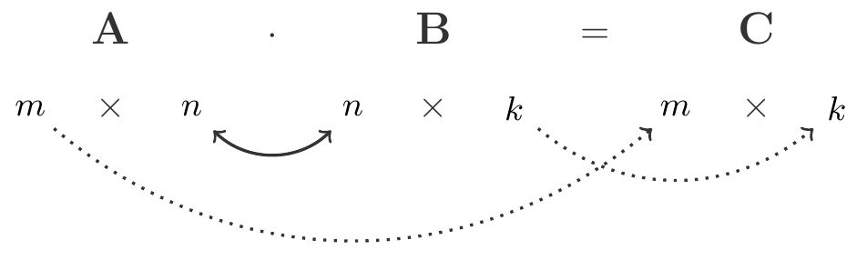
7.2.2 Eigenschaften des Matrixprodukts
In Beispiel 7.7 hatten wir: \[
\begin{gathered}
\begin{array}{ccccc}
\mathbf A & \cdot & \mathbf B & = & \mathbf C \\
4\times 3 & \leftrightarrow & 3\times 4 & & 4 \times 4
\end{array}
\end{gathered}
\] Wir können mit den Angaben dieses Beispiels auch das Produkt \(\mathbf
B\cdot \mathbf
A\) berechnen. \[
\begin{gathered}
\begin{array}{ccccc}
\mathbf B & \cdot & \mathbf A & = & \mathbf D \\
3\times 4 & \leftrightarrow & 4\times 3 & & 3 \times 3
\end{array}
\end{gathered}
\] Das Ergebnis ist allerdings eine andere Matrix als \(\mathbf C\), nämlich: \[
\begin{gathered}
\mathbf B\cdot \mathbf A=\mathbf D=\left(\begin{array}{rrr}
18 & 9 & 2\\
7 & 12 & 4\\
25 & 22 & 7
\end{array}
\right)
\end{gathered}
\] Nun ist klar, dass wir hier ein anderes Ergebnis erhalten müssen. Das liegt an der Art und Weise, wie wir das Produkt bilden, die in diesem Beispiel dazu führt, dass \(\mathbf A\mathbf B\) und \(\mathbf B\mathbf A\) von unterschiedlicher Ordnung sein werden, und damit notwendigerweise \(\mathbf A\mathbf B\ne
\mathbf B\mathbf A\). Aber, was wenn wir das Produkt zweier quadratischer Matrizen gleicher Ordnung bilden?
Wenn \(\mathbf A\) und \(\mathbf B\) von gleicher Ordnung \(n\times n\) sind, dann sind auch \(\mathbf A\mathbf B\) und \(\mathbf B\mathbf A\) von der Ordnung \(n\times n\). Dennoch gilt im Allgemeinen aber: \(\mathbf
A\mathbf B\ne \mathbf B\mathbf A\) !
Satz 7.8 Das Produkt von Matrizen ist im Allgemeinennicht kommutativ. D.h. \[
\begin{gathered}
\mathbf A\cdot \mathbf B\ne \mathbf B\cdot \mathbf A.
\end{gathered}
\]
Die Tatsache, dass im Allgemeinen das Kommutativgesetz nicht gilt, macht das Rechnen mit Matrizen doch etwas mühsamer.
Es gibt aber Ausnahmen von dieser Regel. Die wichtigste Ausnahme ist die Einheitsmatrix (siehe 7.1). Sie ist das neutrale Element der Matrixmultiplikation und es gilt immer: \[
\begin{gathered}
\mathbf A\cdot \mathbf I=\mathbf I\cdot \mathbf A=\mathbf A.
\end{gathered}
\tag{7.3}\] Mysteriöserweise gibt es aber zu einer gegebenen quadratischen Matrix \(\mathbf A\) gleich unendlich viele weitere Matrizen, die mit \(\mathbf
A\) kommutieren, und denen man das nicht so ohne weiteres von außen ansehen kann. Z.B. \[
\begin{gathered}
\mathbf A=\left(\begin{array}{cc} 1& 2 \\3 &
4\end{array}\right),\qquad
\mathbf C=\left(\begin{array}{rr}
5 & 6\\
9 & 14
\end{array}\right),\quad \mathbf A\mathbf C=\mathbf C\mathbf A=
\left(\begin{array}{rr}
23 & 34\\
51 & 74
\end{array}\right).
\end{gathered}
\] Abgesehen von dieser gewöhnungsbedürftigen Merkwürdigkeit besitzt das Matrixprodukt doch Eigenschaften, die wir vernünftigerweise von einem Produkt erwarten:
Satz 7.9 (Assoziativgesetz) Es seien \(\mathbf A,\, \mathbf B\) und \(\mathbf C\) Matrizen, die miteinander multiplizierbar sind. Dann \[
\begin{gathered}
(\mathbf A\cdot \mathbf B)\cdot \mathbf C = \mathbf A\cdot
(\mathbf B\cdot \mathbf C).
\end{gathered}
\tag{7.4}\]
Dieses Gesetz sagt aus, dass es beim Multiplizieren von mehr als zwei Matrizen auf die Klammerung nicht ankommt. Beachten Sie aber, dass dabei die Reihenfolge der Faktoren nicht verändert wird. Es wird lediglich festgelegt, welche Multiplikation zuerst ausgeführt wird, welche als zweite, usw.
Aus dem Assoziativgesetz folgt, dass man von quadratischen Matrizen Potenzen \(\mathbf A^2:=\mathbf A\cdot
\mathbf A\), \(\mathbf A^3:=\mathbf A\cdot \mathbf A\cdot \mathbf A\), usw., bilden kann. Wäre nämlich \((\mathbf A\cdot \mathbf
A)\cdot\mathbf A\not=
\mathbf A\cdot(\mathbf A\cdot \mathbf A)\), dann wäre \(\mathbf A^3\) zweideutig und daher nicht definiert.
Außerdem gilt ein Distributivgesetz, genauer gesagt, sogar zwei davon. Der Grund dafür, dass es gleich zwei sind, ist natürlich das Fehlens des Kommutativgesetzes.
Satz 7.10 (Distributivgesetze) Sind \(\mathbf A,\mathbf B,\mathbf C\) Matrizen und sind die Produkte \(\mathbf A\mathbf B, \mathbf A\mathbf C\) und \(\mathbf B\mathbf C\) möglich, dann gilt für die Multiplikation der Matrix \(\mathbf A\) von links an die Summe \(\mathbf B+\mathbf C\): \[
\begin{gathered}
\mathbf A(\mathbf B+\mathbf
C)=\mathbf A\mathbf B+\mathbf A\mathbf C.
\end{gathered}
\tag{7.5}\] Entsprechend gilt für die Multiplikation von rechts: \[
\begin{gathered}
(\mathbf A+\mathbf B)\mathbf C=\mathbf A\mathbf C+\mathbf B\mathbf C.
\end{gathered}
\tag{7.6}\]
Es ist wichtig, genau zu verstehen, was (7.5) besagt. Von links nach rechts gelesen: wir dürfen die Klammer auflösen. Von rechts nach links gelesen: wir dürfen einen gemeinsamen Faktor von zwei oder mehreren Produkten herausheben. Dieser Faktor muss aber in allen Produkten auf der gleichen Seite stehen.
Die folgenden drei Aufgaben sind nicht nur zum Üben gedacht, sie zeigen auch ein paar weitere seltsame Eigenschaften des Matrixprodukts.
Lösung: Mit dem Falk-Schema finden Sie: \[
\begin{gathered}
\mathbf A\mathbf B=\left(\begin{array}{ccc}
0 & 0 & 0\\
0 & 0 & 0\\
0 & 0 & 0
\end{array}\right)=\mathbf{0}
\end{gathered}
\] □
Das ist eine weitere merkwürdige Eigenschaft des Matrixprodukts. Wenn für zwei reelle Zahlen \(a,b\) gilt: \(ab=0\), dann können wir sicher sein, dass einer der Faktoren (oder beide) Null sind. Bei Matrizen gilt diese Regel nicht mehr.
Das hat Konsequenzen beim Lösen von Gleichungen, einem Thema, das wir in Kürze genauer behandeln werden. Wenn \(a,b\) und \(x\ne 0\) reelle Zahlen sind, dann gilt bekanntlich die Kürzungsregel: \[
\begin{gathered}
ax=bx\implies a=b,\qquad\text{wenn }x\ne 0.
\end{gathered}
\] Bei Matrizen gilt diese Regel im allgemeinen nicht.
Lösung: Mit dem Falk-Schema finden Sie \(\mathbf A^2=\mathbf A\), daraus folgt aber, dass \(\mathbf A^n=\mathbf A\) für \(n=1,2,\ldots\). Eine Matrix mit dieser Eigenschaft heißt idempotent. □
Auch die folgende Aufgabe zeigt eine Besonderheit, die wir so vom Rechnen mit Zahlen nicht kennen.
Wir beschließen diesen Abschnitt mit einer weiteren wichtigen Eigenschaft des Matrixprodukts:
Satz 7.15 Es seien \(\mathbf A\) und \(\mathbf B\) zwei Matrizen von solcher Ordnung, dass das Produkt \(\mathbf A\mathbf B\) gebildet werden kann. Dann gilt: \[
\begin{gathered}
{(\mathbf A\mathbf B)}^\top={\mathbf
B}^\top {\mathbf A}^\top.
\end{gathered}
\]
Wir überlassen es interessierten Leserinnen und Lesern, diese Beziehung anhand eines Beipiels zu überprüfen.
7.2.3 Spezielle Produkte
Ein wichtiger Spezialfall der Matrixmultiplikation ist die Multiplikation einer Matrix mit einem Spaltenvektor. Es sollte völlig klar sein, dass man von rechts an eine Matrix immer einen (passenden) Spaltenvektor multiplizieren kann. Das Resultat ist wieder ein Spaltenvektor. \[
\begin{gathered}
\begin{array}{ccccc}
\mathbf A & \cdot & \mathbf b & = & \mathbf c \\
m\times n & \leftrightarrow &n\times 1 & & m
\times 1
\end{array}
\end{gathered}
\]
Das Produkt Matrix \(\times\) Spaltenvektor ist uns schon in Kapitel 6 begegnet. Wir erinnern uns an die allgemeine Form eines linearen Gleichungssystems: \[
\begin{gathered}
\begin{array}{rcrcrcr}
a_{11}x_1 &+& a_{12}x_2 &+\cdots+& a_{1n}x_n &=& b_1 \\
a_{21}x_1 &+& a_{22}x_2 &+\cdots+& a_{2n}x_n &=& b_2 \\
\vdots && \vdots && \vdots && \vdots\\
a_{m1}x_1 &+& a_{m2}x_2 &+\cdots+& a_{mn}x_n &=& b_m \\
\end{array}
\end{gathered}
\] Bei genauerer Betrachtung erkennen Sie, dass die linken Seiten der Gleichungen tatsächlich Summen von Produkten sind. Aber genau so bilden wir das Matrixprodukt! Das bedeutet: Jedes lineare Gleichungssystem lässt sich unter Verwendung der Matrixmultiplikation als Matrixgleichung \[
\begin{gathered}
\mathbf A\cdot \mathbf x=\mathbf b
\end{gathered}
\tag{7.7}\] schreiben. Dabei bezeichnet \(\mathbf A\) die Koeffizientenmatrix, \(\mathbf x\) den Vektor der unbekannten Variablen und \(\mathbf b\) den Vektor der rechten Seite des Gleichungssystems.
Ein weiterer wichtiger Sonderfall der Matrixmultiplikation ist die Multiplikation eines Zeilenvektors mit einer Matrix. Man mache sich wieder klar, dass lediglich ein Zeilenvektor von links an eine Matrix mit mehr als einer Zeile multipliziert werden kann. Das Ergebnis ist wieder ein Zeilenvektor: \[
\begin{gathered}
\begin{array}{ccccc}
{\mathbf a}^\top & \cdot & \mathbf B &=& {\mathbf c}^\top \\
1\times m & \leftrightarrow &m \times n &&
1 \times n
\end{array}
\end{gathered}
\tag{7.8}\]
Einen letzten Sonderfall wollen wir noch kurz erwähnen. Wenn in (7.8) die Matrix \(\mathbf B\) nur eine Spalte hat, dann bilden wir das Produkt eines Zeilenvektors mit einem Spaltenvektor: \[
\begin{gathered}
\begin{array}{ccccc}
{\mathbf a}^\top & \cdot & \mathbf b &=& \mathbf c \\
1\times m & &m \times 1 &&
1 \times 1
\end{array}
\end{gathered}
\tag{7.9}\] Das Ergebnis ist eine Matrix der Ordnung \(1\times 1\), also eine gewöhnliche Zahl.
Musteraufgabe 7.19 Berechnen Sie das Produkt \(\displaystyle
\left(\begin{array}{ccc}1 & 2 & 3\end{array}\right)
\left(\begin{array}{r}4\\-1\\2\end{array}\right).\)
Dieses spezielle Produkt wird Ihnen wahrscheinlich unter dem Namen Skalarprodukt von Vektoren bekannt sein.
Ein wichtiger Spezialfall der Multiplikation eines Zeilenvektors mit einem Spaltenvektor liegt vor, wenn die beiden Faktoren gleich sind: \[
\begin{gathered}
{\mathbf a}^\top \mathbf a=a_1^2+a_2^2+\ldots+a_n^2.
\end{gathered}
\tag{7.10}\] Dieses Produkt liefert also die Summe der Komponentenquadrate eines Vektors!
7.3 Matrizen in der Planungsrechnung
7.3.1 Grundgleichung der Bedarfsplanung
Eine der wichtigsten wirtschaftlichen Anwendungen der Matrizenrechnung ist die Bedarfsplanung. Dabei haben Matrizen die Bedeutung von Bedarfsmatrizen, das sind Mengengerüste in Tabellenform, welche die verwendete Produktionstechnologie repräsentieren. Diese Technologie ist linear, damit meinen wir, dass eine Erhöhung der Inputs um einen Faktor \(\alpha\) eine Outputerhöhung um denselben Faktor bewirkt.
Wir knüpfen im folgenden Einführungsbeispiel an den Abschnitt 6.3.2 an, in dem wir den Begriff der Bedarfsvektoren erklärt haben. Man kann die Berechnungen, die mit Bedarfsvektoren einhergehen, sehr einfach und übersichtlich in Matrixschreibweise darstellen.
Ein Möbelhaus bietet unter anderem auch zwei Arten von Bücherregalen zum Selbstbau an. Regaltyp A hat eine Höhe von 200 cm, Typ B ist die kleinere Variante mit einer Höhe von 110 cm. Für Typ A werden pro Stück 5 \(m^2\) furnierte Platten verarbeitet, für Typ B braucht man 3 \(m^2\) Platten. Die Fertigung (Zuschnitt der Platten, Bohrungen und Verpackung) erfolgt vollautomatisch. Bei Typ A nimmt die Fertigung 8 Minuten Maschinenzeit in Anspruch, bei Typ B 6 Minuten.
Wir haben den Inputvektor für den Output von 50 Regalen A und 20 Regalen B durch eine Linearkombination \[
\begin{gathered}
50\mathbf a+20\mathbf b=
50\left(\begin{array}{c}5\\8
\end{array}\right)+
20\left(\begin{array}{c}3\\6
\end{array}\right)=
\left(\begin{array}{c}310\\520
\end{array}\right).
\end{gathered}
\] berechnet. Man kann diesen Rechenschritt auch in Matrixschreibweise darstellen. Dazu fassen wir die herzustellenden Mengen in einem Outputvektor\(\mathbf x\) zusammen: \[
\begin{gathered}
\mathbf x=\left(\begin{array}{c}
50\\20
\end{array}\right).
\end{gathered}
\] Weiters bilden wir aus den Bedarfsvektoren eine Bedarfsmatrix so, dass jeder Bedarfsvektor zu einer Spalte dieser Matrix wird: \[
\begin{gathered}
\mathbf A=\left(
\begin{array}{cc}
5 & 3\\
8 & 6
\end{array}\right).
\end{gathered}
\] Der benötigter Inputvektor (Inputmengen) \(\mathbf b\) ergibt sich nun als einfaches Produkt der Bedarfsmatrix mit dem Outputvektor: \[
\begin{gathered}
\mathbf b=\mathbf A\mathbf x=
\left(
\begin{array}{cc}
5 & 3\\
8 & 6
\end{array}\right)\left(\begin{array}{c}
50\\20
\end{array}\right) = \left(\begin{array}{c}
310\\520
\end{array}\right).
\end{gathered}
\]
Beispiel 7.21
Ein Unternehmen fertigt aus den vier Anfangsprodukten \(A_1, A_2,
A_3\) und \(A_4\) drei Endprodukte \(B_1,B_2\) und \(B_3\). Um 1 \(B_1\) herzustellen, werden 3 \(A_1\), 2 \(A_2\) und 4 \(A_4\) benötigt. Bei der Erzeugung von 1 \(B_2\) werden 2 \(A_1\), 4 \(A_2\), 2 \(A_3\) und 1 \(A_4\) verarbeitet. Um 1 \(B_3\) herzustellen benötigt man 1 \(A_2\) und 2 \(A_3\). Dieses Mengengerüst hat die Form von einer Bedarfstabelle: \[
\begin{gathered}
\begin{array}{c|ccc}
& B_1 & B_2 & B_3\\
\hline
A_1 & 3 & 2 & 0\\
A_2 & 2 & 4 & 1\\
A_3 & 0 & 2 & 2\\
A_4 & 4 & 1 & 0
\end{array}\quad\longrightarrow: \mathbf A=
\left(\begin{array}{ccc}
3 & 2 & 0\\
2 & 4 & 1\\
0 & 2 & 2\\
4 & 1 & 0
\end{array}\right)
\end{gathered}
\] Die aus der Bedarfstabelle erstellte Matrix \(\mathbf A\) nennt man Bedarfsmatrix. Sie beschreibt mengenmäßig die Transformation der Inputs\(A_1, A_2, A_3\) und \(A_4\) in die Outputs \(B_1,B_2\) und \(B_3\). Die einzelnen Spalten sind die Bedarfsvektoren der Endprodukte.
Die Grundaufgabe der Bedarfsplanung, die Teilebedarfsrechnung, lautet nun: wenn ein konkreter Produktionsauftrag vorliegt, welche Inputmengen sind erforderlich, um diesen Auftrag zu erfüllen?
Nehmen wir beispielsweise an, es sollen 10 Einheiten \(B_1\), 15 Einheiten \(B_2\) und 20 Einheiten \(B_3\) geliefert werden. Wir fassen diese Mengen in einem Outputvektor \(\mathbf x\) zusammen: \[
\begin{gathered}
\mathbf x=\left(\begin{array}{r}10\\15\\20\end{array}\right).
\end{gathered}
\] Wir können nun sofort sagen, wieviel wir an \(A_1\) brauchen werden, um diesen Auftrag zu erfüllen. Die Informationen dazu finden sich in der 1. Zeile der Bedarfsmatrix \(\mathbf A\) und im Outputvektor \(\mathbf x\): \[
\begin{gathered}
\text{Bedarf an $A_1$: }\quad 3\cdot 10+2\cdot 15+0\cdot 20=60
\end{gathered}
\] Das ist offenbar das Produkt der 1. Zeile von \(\mathbf A\) mit dem Vektor \(\mathbf x\). In analoger Weise errechnet sich der Bedarf an \(A_2,A_3\) und \(A_4\) als Produkt der 2., 3. und 4. Zeile von \(\mathbf A\) mit \(\mathbf x\). Kurz, die Inputmengen sind die Komponenten des Vektors \(\mathbf b\), der sich als Produkt der Bedarfsmatrix mit dem Outputvektor ergibt: \[
\begin{gathered}
\mathbf b=\mathbf A\mathbf x=
\left(\begin{array}{ccc}
3 & 2 & 0\\
2 & 4 & 1\\
0 & 2 & 2\\
4 & 1 & 0
\end{array}\right)\left(\begin{array}{r}10\\15\\20\end{array}
\right)=\left(\begin{array}{r}60\\100\\70\\55\end{array}\right).
\end{gathered}
\]
Die in den letzten beiden Beispielen identifizierte Beziehung zwischen Bedarfsmatrix, Output- und Inputvektoren ist so bedeutsam, dass wir festhalten:
Definition 7.22 (Grundgleichung der Bedarfsplanung) Es sei \(\mathbf x\) der Outputvektor, \(\mathbf A\) die Bedarfsmatrix. Dann sind die erforderlichen Inputs \(\mathbf b\): \[
\begin{gathered}
\mathbf b=\mathbf A\cdot \mathbf x.
\end{gathered}
\tag{7.11}\]
Musteraufgabe 7.23 Ein Unternehmen fertigt unter anderem elektronische Baugruppen \(B_1, B_2\) und \(B_3\). Dazu werden Kondensatoren (C) und Widerstände (R) benötigt. Der Bedarf an Kondensatoren und Widerständen sowie die verfügbaren Lagerbestände sind der folgenden Tabelle zu entnehmen:
Ein Auftrag sieht vor, 100 St. von \(B_1\), 150 St. von \(B_2\) und 120 St. von \(B_3\) zu liefern.
Kann der Auftrag mit den vorhandenen Lagerbeständen ausgeführt werden?
Wenn ja, was ist der Lagerbestand nach Ausführung des Auftrages?
Lösung: Wir berechnen den benötigten Input mit Hilfe der Grundgleichung (7.11) der Bedarfsplanung. Es bezeichne \(\mathbf A\) die Bedarfsmatrix, \(\mathbf x\) den Outputvektor und \(\mathbf b\) den Inputvektor. Die Grundgleichung lautet \(\mathbf A\mathbf x=\mathbf b\), und in Zahlen \[
\begin{gathered}
\mathbf b=\left(
\begin{array}{rrr}
5 & 2 & 9\\
2 & 1 & 6
\end{array}\right)
\left(\begin{array}{r}
100\\
150\\
120
\end{array}\right)
=
\left(\begin{array}{r}
1880\\
1070
\end{array}\right).
\end{gathered}
\] Das ist der benötigte Inputvektor für den geplanten Output. Wir vergleichen nun die vorhandenen Lagerbestände mit dem benötigten Input: \[
\begin{gathered}
\text{Anfangsbestand } \mathbf a=
\left(\begin{array}{r}
2000\\
1200
\end{array}\right)
,\quad\text{Endbestand } \mathbf e =\mathbf a-\mathbf b =
\left(\begin{array}{r}
120\\
130
\end{array}\right).
\end{gathered}
\] Der Auftrag kann ausgeführt werden, da \(\mathbf e\ge \mathbf{0}\), dh. es gibt keine Fehlmengen.
7.3.2 Kostenseite der Bedarfsplanung
Ein Hersteller produziert die Produkte \(B_1,B_2,\ldots,B_n\) und benötigt hierzu die Rohstoffe \(A_1,A_2,\ldots,A_r\). Die Bedarfsmatrix lautet \[
\begin{gathered}
\begin{array}{c|cccc}
&B_1&B_2&\ldots &B_n\\
\hline
A_1&a_{11}&a_{12}& \ldots&a_{1n}\\
A_2&a_{21}&a_{22}& \ldots&a_{2n}\\
\vdots&\vdots&\vdots&\ddots&\vdots\\
A_r&a_{r1}&a_{r2}&\ldots&a_{rn}\\
\end{array}
\quad\longrightarrow :\quad
\mathbf A=\left(\begin{array}{cccc}
a_{11}&a_{12}& \ldots&a_{1n}\\
a_{21}&a_{22}& \ldots&a_{2n}\\
\vdots&\vdots&\ddots&\vdots\\
a_{r1}&a_{r2}&\ldots&a_{rn}
\end{array}\right)
\end{gathered}
\] Es sei \({\mathbf p}^\top =(p_1,p_2,\ldots,p_r)\) der Vektor der Rohstoffpreise und der Vektor \(\mathbf x\) enthalte die geplanten Outputmengen, d.h. \({\mathbf x}^\top =(x_1,x_2,\ldots,x_n)\).
Wir stellen nun die folgenden Fragen:
Wie hoch sind die Gesamtkosten des Auftrags repräsentiert durch \(\mathbf x\)?
Wie hoch sind die Produktionskosten der einzelnen Produkte ?
Natürlich ist es möglich diese Fragen sehr einfach ohne Zuhilfenahme der Matrizenrechnung beantworten. Uns kommt es aber darauf an, wie man mit Matrizenrechnung eine übersichtliche Darstellung der Antwort erhält.
Man kann die Gesamtkosten durch ein einfaches Matrixprodukt darstellen. Wie wir wissen, erhalten wir den Mengenvektor \(\mathbf b\) der für die Produktion \(\mathbf x\) benötigten Rohstoffe durch \[
\begin{gathered}
\mathbf b=\mathbf A\cdot \mathbf x.
\end{gathered}
\] Andererseits ergeben sich die Kosten \(K\) für die verarbeiteten Rohstoffmengen \(\mathbf b\) durch das Produkt \[
\begin{gathered}
K=p_1b_1+p_2b_2+\cdots+ p_rb_r= {\mathbf p}^\top \cdot \mathbf b.
\end{gathered}
\] Daraus folgt durch Einsetzen der Gleichungen ineinander und aus dem Assoziativgesetz: \[
\begin{gathered}
K={\mathbf p}^\top \cdot \mathbf b={\mathbf p}^\top \cdot
(\mathbf A\cdot \mathbf x)=({\mathbf p}^\top \cdot \mathbf
A)\cdot \mathbf x.
\end{gathered}
\tag{7.12}\] Dies ist die Matrixgleichung, die die Gesamtkosten darstellt.
Der Zeilenvektor \({\mathbf c}^\top ={\mathbf p}^\top \cdot \mathbf A\) hat eine einfache und wichtige Interpretation. Er enthält die Kosten der einzelnen Produkte: \[
\begin{gathered}
{\mathbf p}^\top \cdot \mathbf A= (p_1,p_2,\ldots,p_r)
\left( \begin{array}{ccc}
a_{11} & \ldots & a_{1n} \\
a_{21} & \ldots & a_{2n} \\
\vdots & \ddots & \vdots \\
a_{r1} & \ldots & a_{rn}
\end{array}\right)=(c_1,c_2,\ldots,c_n)
={\mathbf c}^\top .
\end{gathered}
\]
Musteraufgabe 7.24 Ein Hersteller produziert zwei Produkte \(B_1\) und \(B_2\). Er benötigt dazu Rohstoffe \(A_1, A_2\) und \(A_3\). Die Produktion erfolgt an zwei verschiedenen Standorten \(S_1\) und \(S_2\). An den beiden Standorten wird zwar dieselbe Produktionstechnologie eingesetzt, aber die Einstandspreise der Rohstoffe sind an diesen Standorten verschieden. Der Bedarf an Rohstoffen sowie deren Einstandspreise in \(S_1\) und \(S_2\) sind gegeben durch:
(a) Die Produktionskosten an den beiden Standorten betragen: \[
\begin{gathered}
\text{Kosten in $S_1$:}\quad {\mathbf c_1}^\top =
{\mathbf p_1}^\top \cdot \mathbf
A=
(10,2,3)
\left(\begin{array}{cc}
3 & 4\\
2 & 1\\
4 & 6
\end{array}
\right)=(46,60).\\
\text{Kosten in $S_2$:}\quad {\mathbf c_2}^\top =
{\mathbf p_2}^\top \cdot \mathbf
A=
(9,3,4)
\left(\begin{array}{cc}
3 & 4\\
2 & 1\\
4 & 6
\end{array}
\right)=(49,63).
\end{gathered}
\] (b) Um die Gesamtkosten zu berechnen, müssen wir von rechts mit dem Outputvektor \[
\begin{gathered}
\mathbf x=\left(\begin{array}{c}500\\200\end{array}\right)
\end{gathered}
\] multiplizieren. Das ergibt: \[
\begin{gathered}
K_1=({\mathbf p_1}^\top \cdot \mathbf A)\cdot \mathbf x=(46,60)
\left(\begin{array}{c}500\\200\end{array}\right)=35000,\\
K_2=({\mathbf p_2}^\top \cdot \mathbf A)\cdot \mathbf x=(49,63)
\left(\begin{array}{c}500\\200\end{array}\right)=37100.
\end{gathered}
\] □
Musteraufgabe 7.25 In einem Unternehmen werden die Produkte \(P_1,P_2\) und \(P_3\) mittels zweier Maschinen \(M_1\) und \(M_2\) hergestellt. Die erforderlichen Maschinenzeiten pro Stück (in Minuten) sowie die Maschinenkosten sind der folgenden Tabelle zu entnehmen:
Ein Auftrag erfordert die Lieferung von 200 Stück \(P_1\), 100 Stück \(P_2\) und 180 Stück \(P_3\). Berechnen Sie die Gesamtkosten dieses Auftrags.
Lösung: Wir bezeichnen mit \(\mathbf A\) die Bedarfsmatrix, mit \(\mathbf x\) den Outputvektor und mit \(\mathbf k\) den Kostenvektor der Maschinenzeiten: \[
\begin{gathered}
\mathbf A=\left(\begin{array}{rrr}
20 & 4 & 10\\5 & 8 & 12
\end{array}\right),\quad
\mathbf x=\left(\begin{array}{r}200\\100\\180\end{array}\right),\quad
\mathbf k=\frac{1}{60}\left(\begin{array}{r}150\\120\end{array}\right).
\end{gathered}
\] Beachten Sie, dass wir hier mit Kosten/Minute rechnen. Die Gesamtkosten des Auftrags sind dann \[
\begin{aligned}
c&={\mathbf k}^\top \cdot \mathbf A\cdot \mathbf x\\
&=\frac{1}{60}\left(\begin{array}{rr}150 & 120\end{array}\right)
\left(\begin{array}{rrr}
20 & 4 & 10\\5 & 8 & 12
\end{array}\right)\left(\begin{array}{r}200\\100\\180\end{array}\right)\\
&=\frac{1405200}{60}=23420\text{ GE}.
\end{aligned}
\] □
Musteraufgabe 7.26 In einem Unternehmen werden aus Bauteilen \(A_1\) und \(A_2\) Baugruppen \(B_1\) und \(B_2\) gefertigt, die in einem weiteren Verarbeitungsschritt zu Geräten \(E_1, E_2\) und \(E_3\) montiert werden. Ein Lieferauftrag erfordert die Herstellung von 100 Stück \(E_1\), 200 Stück \(E_2\) und 50 Stück \(E_3\). Über den Mengenbedarf in den beiden Produktionsstufen ist soviel bekannt:
Eine kurze Rechnung überzeugt den Produktionsleiter, dass dieser Auftrag mit den vorhandenen Lagerbeständen nicht durchgeführt werden kann. Als kurzfristiger Ausweg bietet sich lediglich die Möglichkeit, fertige Baugruppen von einem Konkurrenzunternehmen zuzukaufen. Dieses verrechnet allerdings Stückpreise von 12 bzw 15 GE für \(B_1\) bzw. \(B_2\), während die Herstellung von \(B_1\) und \(B_2\) lediglich 10 bzw. 12 GE/St. kostet. Welche Mehrkosten ergeben sich, wenn der Lagerbestand zur Gänze verbraucht wird?
Lösung: Bedarfsmatrix und gewünschter Outputvektor sind: \[
\begin{gathered}
\mathbf A=\left(\begin{array}{rrr}
5 & 2 & 1\\
0 & 10 & 20
\end{array}\right),
\quad \mathbf x=\left(\begin{array}{r}100\\200\\50
\end{array}\right).
\end{gathered}
\] Für den Output \(\mathbf x\) benötigen wir an Baugruppen \(B_1\) und \(B_2\): \[
\begin{gathered}
\mathbf q=\mathbf A\mathbf x=\left(\begin{array}{rrr}
5 & 2 & 1\\
0 & 10 & 20
\end{array}\right)
\left(\begin{array}{r}
100\\200\\50
\end{array}\right)
=
\left(\begin{array}{r}
950\\3000
\end{array}
\right).
\end{gathered}
\] Andererseits müssen wir uns fragen, welche Mengen \(b_1\) und \(b_2\) der Baugruppen \(B_1\) und \(B_2\) aus den vorhandenen Lagerbeständen hergestellt werden können. Diese Frage führt auf die Lösung eines Gleichungssystems: \[
\begin{gathered}
\left(
\begin{array}{cc}
4 & 6 \\
7 & 0
\end{array}
\right)
\cdot
\left(
\begin{array}{r}
b_1\\
b_2
\end{array}
\right)=
\left(
\begin{array}{r}
14\,000 \\
350
\end{array}
\right)
\quad
\implies
\quad
\begin{array}{rcrcr}
4b_1 &+& 6b_2 &=& 14000\\
7b_1 & & &=& 350
\end{array}
\end{gathered}
\] Dieses Gleichungssystem hat die Lösung \(b_1=50\), \(b_2=2300\). Daher lautet der produzierbare Outputvektor an Baugruppen \[
\begin{gathered}
\mathbf b=\left(\begin{array}{r}50\\2300\end{array}
\right).
\end{gathered}
\] Aus der Differenz erhalten wir die benötigten Zukaufsmengen: \[
\begin{gathered}
\mathbf q-\mathbf b=\left(\begin{array}{r}900\\700\end{array}\right).
\end{gathered}
\] Die dadurch entstehenden Mehrkosten berechnen wir, indem wir den Vektor der Preisdifferenz \[
\begin{gathered}
\Delta\mathbf p=\left(\begin{array}{r}2\\3\end{array}\right)
\end{gathered}
\] mit dem Vektor der Zukaufsmengen multiplizieren: \[
\begin{gathered}
c=\Delta {\mathbf p}^\top \cdot (\mathbf q-\mathbf b)
= 2\cdot 900+3\cdot 700 =3900.
\end{gathered}
\] □
7.3.3 Mehrstufige Produktionsprozesse
In der Praxis sind Produktionsprozesse nicht so einfach strukturiert wie in den bisherigen Beispielen, vielmehr umfassen sie mehrere Prozessstufen, in welchen Zwischenprodukte aus Inputs gefertigt werden, die aus technologisch vorgelagerten Stufen stammen. Die Outputs einer Stufe werden in einer oder mehreren nachgelagerten Prozessstufen weiterverarbeitet, bis schließlich am Ende der Kette das oder die fertigen Endprodukte herauskommen. Für jede Fertigungsstufe ist der mengenmäßige Zusammenhang zwischen den Inputs und den Outputs bekannt und durch eine Bedarfsmatrix gegeben.
Welche Mengen an Anfangsprodukten müssen vorhanden sein, um einen gegebenen Output von Endprodukten zu produzieren?
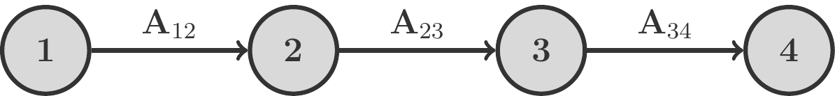
Beispiel 7.27 (Ein dreistufiger Prozess)
Betrachten wir als Beispiel einen dreistufigen Prozess, dessen Stufen strikt in einer Reihe angeordnet sind. Eine Anordnung dieser Art wird auch Flow Shop genannt. Aus den \(m\) Anfangsprodukten \(A_1,\ldots,A_m\) werden in der ersten Stufe \(n\) Zwischenprodukte \(P_1,\ldots,P_n\) gefertigt. Die zugehörige Bedarfsmatrix sei \(\mathbf A_{12}\). Aus \(P_1,\ldots,P_n\) stellt man in der zweiten Stufe \(r\) Zwischenprodukte \(Q_1,\ldots,Q_r\) her, die Bedarfsmatrix dieser Stufe nennen wir \(\mathbf A_{23}\). Schließlich werden aus \(Q_1,\ldots,Q_r\) die \(s\) Endprodukte \(E_1,\ldots,E_s\) hergestellt. Die Bedarfsmatrix der dritten Stufe sei \(\mathbf A_{34}\).
Schematisch kann man diesen Prozess so darstellen:
\[
\begin{gathered}
\begin{array}{|cccc|}
\hline\rowcolor{mgray}\rule{0pt}{11pt}
\text{Stufe} & \text{Inputs}
& \text{Outputs} & \text{Bedarfsmatrix}\\
\hline
\rule{0pt}{13pt}
1\to 2
&
A_1,\ldots, A_m & P_1,\ldots, P_n & \mathbf A_{12}\\
2\to 3 & P_1,\ldots, P_n & Q_1,\ldots, Q_r & \mathbf A_{23}\\
3\to 4 & Q_1,\ldots, Q_r & E_1,\ldots, E_s& \mathbf A_{34}\\[2pt]
\hline
\end{array}
\end{gathered}
\] Gegeben sei nun ein Auftragsvektor \(\mathbf x\), und wir suchen die erforderlichen Inputs der 1. Stufe. Diese Mengen fassen wir in einem Vektor \(\mathbf a\) zusammen.
Um \(\mathbf a\) zu finden, arbeiten wir den Fertigungsprozess von rechts nach links ab. Wir sehen uns also zuerst die letzte Stufe des Produktionsprozesses an. Die Inputs an \(Q_1,\ldots,Q_r\) der letzten Stufe, wir fassen sie in einem Vektor \(\mathbf q\) zusammen, ergeben sich nach der Grundgleichung der Bedarfsplanung aus dem Produkt: \[
\begin{gathered}
\mathbf q=\mathbf A_{34}\cdot\mathbf x
\end{gathered}
\tag{7.13}\] Nun ist \(\mathbf q\) zugleich der Outputvektor der 2. Stufe. Um dieses \(\mathbf q\) herzustellen, sind Inputmengen \(\mathbf p\) von Produkten \(P_1,\ldots,P_n\) erforderlich, wobei \[
\begin{gathered}
\mathbf p=\mathbf A_{23}\cdot\mathbf q
\end{gathered}
\tag{7.14}\] Wenn \(\mathbf p\) der Output der 1. Stufe ist, dann sind die dazu notwendigen Mengen an \(A_1,\ldots,A_m\) gerade die des Inputvektors \(\mathbf a\): \[
\begin{gathered}
\mathbf a=\mathbf A_{12}\cdot\mathbf p
\end{gathered}
\tag{7.15}\] Wir setzen nun (7.13) in (7.14) ein und das wiederum in (7.15). Dabei nützen wir das Assoziativgesetz der Matrixmultiplikation: \[
\begin{aligned}
\mathbf a=\mathbf A_{12}\mathbf p&=\mathbf A_{12}(\mathbf A_{23}\mathbf q)\\
&=\mathbf A_{12}\mathbf A_{23}(\mathbf A_{34}\mathbf x)\\
&=\mathbf A_{12}\mathbf A_{23}\mathbf A_{34}\mathbf x=\mathbf A\mathbf x
\end{aligned}
\]\(\mathbf A\) bezeichnet die globale Bedarfsmatrix für den mengenmäßigen Zusammenhang zwischen Anfangs- und Endprodukten. Wir stellen fest: \(\mathbf A\) ist das Produkt der Bedarfsmatrizen entlang des einzigen Weges durch das Schema des Prozesses, wobei dieses Matrixprodukt exakt in der technologischen Reihenfolge gebildet wird.
Musteraufgabe 7.28 Aus 3 Anfangsprodukten \(A_1,A_2\) und \(A_3\) werden in erster Stufe Zwischenprodukte \(P_1\) und \(P_2\) gefertigt, aus diesen in zweiter Stufe Zwischenprodukte \(Q_1\) und \(Q_2\) und daraus schließlich in der dritten Stufe die Endprodukte \(E_1,E_2\) und \(E_3\). Die Mengengerüste der Produktionsstufen sind durch folgende Bedarfsmatrizen gegeben: \[
\begin{gathered}
\mathbf A_{12}=\left(\begin{array}{rr}
4 & 0\\
2 & 2\\
0 & 7
\end{array}\right),
\mathbf A_{23}=
\left(\begin{array}{rr}
10 & 20\\
7 & 15
\end{array}\right),
\mathbf A_{34}=
\left(\begin{array}{rrr}
8 & 20 & 10\\
5 & 10 & 15
\end{array}\right).
\end{gathered}
\]
Es soll jeweils 1 Stück von \(E_1\) und \(E_2\) sowie 2 Stück von \(E_3\) hergestellt werden. Welcher Lagerbestand an \(A_1,A_2\) und \(A_3\) muss dafür vorhanden sein?
Lösung: Die globale Bedarfsmatrix lautet \[
\begin{aligned}
\mathbf A\;=\mathbf A_{12}\mathbf A_{23}\mathbf A_{34} &=
\left(\begin{array}{rr}
4 & 0\\
2 & 2\\
0 & 7
\end{array}\right)
\left(\begin{array}{rr}
10 & 20\\
7 & 15
\end{array}\right)
\left(\begin{array}{rrr}
8 & 20 & 10\\
5 & 10 & 15
\end{array}\right)
\\[5pt]
&=\left(\begin{array}{rrr}
720 & 1600 & 1600\\
622 & 1380 & 1390\\
917 & 2030 & 2065
\end{array}\right).
\end{aligned}
\] Um den Outputvektor \({\mathbf x}^\top =(1,1,2)\) produzieren zu können, besteht ein Bedarf an Anfangsprodukten in der Höhe von \[
\begin{gathered}
\mathbf a=\mathbf A\mathbf x =\left(\begin{array}{rrr}
720 & 1600 & 1600\\
622 & 1380 & 1390\\
917 & 2030 & 2065
\end{array}\right).
\left(\begin{array}{r}1\\1\\2\end{array}\right) =
\left(\begin{array}{r}
5520\\
4782\\
7077
\end{array}\right).
\end{gathered}
\] □
Bemerkung 7.29 (Cleveres Rechnen) Das Multiplizieren von Matrizen ist ein aufwendiger Prozess. Wenn \(\mathbf A\) von der Ordnung \(m\times n\) und \(\mathbf B\) von der Ordnung \(n\times k\) ist, dann benötigen wir für das Produkt \(\mathbf
A\cdot\mathbf B\) insgesamt: \[
\begin{gathered}
\text{Multiplikationen: } m\cdot n\cdot k,\quad\text{Additionen:
}m\cdot(n-1)\cdot k
\end{gathered}
\] Ein naheliegender Weg, die Rechnung in Musteraufgabe 7.28 durchzuführen wäre dieser: \[
\begin{gathered}
\mathbf a = (((\mathbf A_{12}\mathbf A_{23})\mathbf A_{34})\mathbf
x)
\end{gathered}
\tag{7.16}\] Übertragen auf ein Falk-Schema, würde das bedeuten, wir rechnen so, dass das Falk-Schema nach rechts gestaffelt wird: \[
\begin{gathered}
\begin{array}{rr|rr|rrr|r}
\mathbf A_{12} & &
{\mathbf A_{23}} & &
{\mathbf A_{34}} & & &
{\mathbf x}\\
\hline
& & & & & & & 1\\
& & 10 & 20 & 8 & 20 & 10 & 1\\
& & 7 & 15 & 5 & 10 & 15 & 2\\
\hline
4 & 0 & 40 & 80 & 720 & 1600 & 1600 & 5520 \\
2 & 2 & 34 & 70 & 622 & 1380 & 1390 & 4782 \\
0 & 7 & 49 & 105 & 917 & 2030 & 2065 & 7077 \\
\end{array}
\end{gathered}
\] D.h., wir multiplizieren zuerst \(\mathbf A_{12}\) mit \(\mathbf A_{23}\). Das Ergebnis wird dann mit \(\mathbf A_{34}\) multipliziert. Schließlich multiplizieren wir das letzte Ergebnis noch mit dem Spaltenvektor \(\mathbf x\). Genau das bedeutet die Klammerung (7.16). Der Rechenaufwand beträgt: 39 Multiplikationen und 21 Additionen.
Der Aufwand lässt sich mehr als halbieren, wenn wir eine andere Klammerung wählen, und das dürfen wir, denn es gilt ja ein Assoziativgesetz. Wir können auch so die Klammern setzen: \[
\begin{gathered}
\mathbf a=(\mathbf A_{12}(\mathbf A_{23}(\mathbf A_{34}\mathbf x)))
\end{gathered}
\] Das würde bedeuten, dass wir das Falk-Schema von oben nach unten staffeln: \[
\begin{gathered}
\begin{array}{rrr|rl}
& & & 1&\\
& & & 1&=\mathbf x\\
& & & 2&\\
\hline
8 & 20 & 10 &48\\
5 & 10 & 15 &45 & =\mathbf A_{34}\mathbf x\\
\hline
& 10 & 20 &1380\\
& 7 & 15 &1011&=\mathbf A_{23}(\mathbf A_{34}\mathbf x)\\
\hline
& 4 & 0 &5520\\
& 2 & 2 &4782&=\mathbf A_{12}(\mathbf A_{23}(\mathbf A_{34}\mathbf x)) \\
& 0 & 7 &7077
\end{array}
\end{gathered}
\] Tatsächlich hat sich der Aufwand praktisch halbiert. Nun benötigen wir nur mehr 16 Multiplikationen und 9 Additionen.
Prozesse mit Verzweigungen
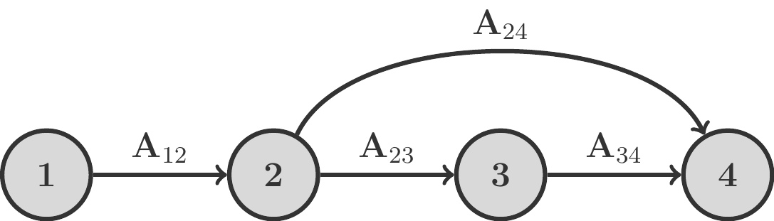
Noch interessanter ist das Problem, wenn der Produktionsprozess Verzweigungen besitzt.
Aus den \(m\) Anfangsprodukten \(A_1,\ldots,A_m\) werden in der ersten Stufe \(n\) Zwischenprodukte \(P_1,\ldots,P_n\) gefertigt. Die zugehörige Bedarfsmatrix sei \(\mathbf A_{12}\).
Aus \(P_1,\ldots,P_n\) stellt man in der zweiten Stufe \(r\) Zwischenprodukte \(Q_1,\ldots,Q_r\) her, die Bedarfsmatrix dieser Stufe nennen wir \(\mathbf A_{23}\).
Schließlich werden aus \(Q_1,\ldots,Q_r\) die \(s\) Endprodukte \(E_1,\ldots,E_s\) hergestellt. Die Bedarfsmatrix der dritten Stufe sei \(\mathbf A_{34}\).
Eine gewisse Anzahl der Zwischenprodukte \(P_i\) wird zusätzlich ohne weitere Verarbeitung in der Endfertigung benötigt. Dieser Bedarf wird durch eine weitere Bedarfsmatrix \(\mathbf A_{24}\) repräsentiert.
Gesucht ist wieder die globale Bedarfsmatrix des Produktionsprozesses.
Schematisch lässt sich die Struktur dieses Produktionsprozesses so darstellen:
Um dieses Problem zu lösen, können wir genauso vorgehen wie vorhin: wir beginnen in der letzten Stufe und arbeiten uns von rechts nach links bis an den Startpunkt des Prozesses vor und berechnen dabei immer den Bedarf an Zwischenprodukten. Dabei haben wir allerdings zu berücksichtigen, dass in der letzten Stufe zwei Materialströme zusammentreffen.
Wir bestimmen alle möglichen Wege durch das Prozessschema: In unserem Beispiel ergibt sich: \[
\begin{gathered}
\begin{array}{lcccccl}
\text{1. Weg: } & 1 & 2 & 3 & 4 & \rightarrow & \mathbf A_{12}\mathbf
A_{23}\mathbf A_{34}\\
\text{2. Weg: } & 1 & 2 & 4 & & \rightarrow & \mathbf A_{12}\mathbf A_{24}\\
\hline
\text{Summe: } & & & & & &\mathbf A_{12}\mathbf A_{23}\mathbf A_{34}+
\mathbf A_{12}\mathbf A_{24}
\end{array}
\end{gathered}
\] Die Bedarfsmatrix \(\mathbf A\), die direkt die Anfangsprodukte mit den Endprodukten verbindet, lautet daher \[
\begin{gathered}
\mathbf A=\mathbf A_{12}\mathbf A_{23}\mathbf A_{34}+ \mathbf A_{12}\mathbf A_{24}=\mathbf A_{12}(\mathbf A_{23}\mathbf A_{34}+\mathbf A_{24}).
\end{gathered}
\] Beachten Sie, dass wir durch Anwenden des Distributivgesetzes\(\mathbf A_{12}\) herausheben konnten und uns auf diese Weise sogar eine Matrixmultiplikation ersparen.
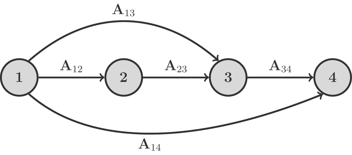
Ein interessanter Sonderfall liegt vor, wenn ein Produktionsfaktor \(A_k\) (z.B. Energie) aus der ersten Stufe auf jeder weiteren Stufe benötigt wird.
Musteraufgabe 7.30 In einem mehrstufigen chemischen Produktionsprozess werden aus zwei Anfangssubstanzen \(A_1\) und \(A_2\) Zwischenprodukte \(P_1\) und \(P_2\) erzeugt. Diese werden zu weiteren Produkten \(Q_1\) und \(Q_2\) verarbeitet, aus denen schließlich in der letzten Phase des Verfahrens die chemischen Stoffe \(E_1,E_2\) und \(E_3\) entstehen. In jeder Phase der Verfahrens wird zur Aufrechterhaltung der chemischen Reaktionen Prozesswärme (in kWh) benötigt. Die Mengengerüste und der Wärmebedarf der Verfahrensschritte sind folgende:
Von den chemischen Substanzen \(E_1,E_2\) und \(E_3\) soll jeweils eine Mengeneinheit erzeugt werden. Welche Mengen Ausgangsstoffen \(A_1\) und \(A_2\) sind dafür erforderlich, was ist der Gesamtbedarf an Prozesswärme?
Lösung: Wir konstruieren einen mehrstufigen Prozess mit Verzweigungen der folgenden Art:
Wir haben es nun mit fünf Bedarfsmatrizen zu tun, wobei die Bedarfsmatrizen \(\mathbf A_{13}\) und \(\mathbf A_{14}\) den Wärmebedarf bei der Produktion der \(Q_i\) und \(E_i\) repräsentieren: \[
\begin{gathered}
\mathbf A_{12}=\left(\begin{array}{cc}
5 & 4\\
2 & 0\\
0 & 3
\end{array}\right),\quad
\mathbf A_{23}=\left(\begin{array}{cc}2 & 0\\1 & 4\end{array}\right),
\quad \mathbf A_{34}=\left(\begin{array}{ccc}1 & 2 & 0\\1 & 0 &
4\end{array}\right)\\[5pt]
\mathbf A_{13}=\left(\begin{array}{rr}10 & 8\\0 & 0\\0 &
0\end{array}\right),\quad
\mathbf A_{14}=\left(\begin{array}{ccc}1 & 2 & 4\\0 & 0 & 0\\0 & 0 &
0\end{array} \right).
\end{gathered}
\] Es gibt drei Wege durch den Prozess mit zugehörigen Bedarfsmatrizen: \[
\begin{gathered}
\begin{array}{ll}
1\to 2\to 3\to 4 & \mathbf A_{12}\mathbf A_{23}\mathbf A_{34}\\
1\to 3\to 4 &\mathbf A_{13}\mathbf A_{34}\\
1\to 4 &\mathbf A_{14}\\
\hline
\text{globale Bedarfsmatrix } \mathbf A=& \mathbf A_{12}\mathbf A_{23}\mathbf
A_{34} +\mathbf A_{13}\mathbf A_{34}+\mathbf A_{14}
\end{array}
\end{gathered}
\] Der Outputvektor ist \({\mathbf x}^\top =(1,1,1)\). Wenn man die Rechnung so durchführt, wie in Bemerkung 7.29 erläutert, dann erhalten wir: \[
\begin{aligned}
\mathbf A\mathbf x&=\mathbf A_{12}\mathbf A_{23}\mathbf A_{34}\mathbf
x + \mathbf A_{13}\mathbf A_{34}\mathbf x+\mathbf A_{14}\mathbf
x\\[5pt]
&=\left(\begin{array}{r}
122\\
12\\
69
\end{array}\right)+\left(\begin{array}{r}
70\\ 0\\ 0\end{array}\right)+
\left(\begin{array}{r}7\\0\\0\end{array}\right)=
\left(\begin{array}{r} 199\\ 12\\ 69\end{array}\right).
\end{aligned}
\] Für diesen Produktionsplan sind daher 199 kWh Prozesswärme, 12 ME von \(A_1\) und 69 ME von \(A_2\) erforderlich. □
7.4 Die Inverse einer Matrix
7.4.1 Der Begriff der inversen Matrix
Inverse Matrizen braucht man, um lineare Matrixgleichungen der Form \(\mathbf
A\mathbf X=\mathbf C\) oder ähnlicher Form lösen zu können.
Bemerkung 7.31 Bevor wir das Problem für Matrizen untersuchen, erinnern wir uns, wie wir solche linearen Gleichungen im Fall von reellen Zahlen lösen.
Will man die Gleichung \(ax=c\) in der Menge der reellen Zahlen lösen, so multipliziert man diese Gleichung mit der Zahl \(b:=\frac{1}{a}\), die die Eigenschaft hat, dass \(b\cdot a=1\). Dadurch erhält man \[
\begin{gathered}
ax=c\;\Rightarrow\;b(ax)=bc \;\Rightarrow \; \underbrace{(ba)}_{=1}x=bc
\;\Rightarrow\; x=bc=\frac{1}{a}\,c.
\end{gathered}
\] Das geht allerdings nur dann, wenn \(b\) existiert, dh. wenn \(a\not= 0\).
Will man die Matrixgleichung \(\mathbf A\mathbf X=\mathbf C\) lösen, dann kann man ähnlich vorgehen. Man sucht eine Matrix \(\mathbf B\) mit der Eigenschaft \(\mathbf B\mathbf A=\mathbf I\). Wir erinnern uns, die Einheitsmatrix \(\mathbf I\) ist das neutrale Element der Matrixmultiplikation, d.h. \(\mathbf I\cdot\mathbf X=\mathbf X\). Wenn es uns gelingt, so eine Matrix \(\mathbf B\) zu finden, dann können wir die Matrixgleichung von links mit diesem \(\mathbf B\) multiplizieren und erhalten: \[
\begin{gathered}
\mathbf B(\mathbf A\mathbf X)=\mathbf B\mathbf C \;\Rightarrow\;
\underbrace{(\mathbf B\mathbf A)}_{=\mathbf I}\mathbf X=\mathbf B\mathbf C \;
\Rightarrow\; \mathbf X=\mathbf B\mathbf C.
\end{gathered}
\tag{7.17}\] Es stellt sich die Frage, unter welchen Voraussetzungen eine Matrix \(\mathbf B\) mit der Eigenschaft \(\mathbf B\mathbf A=\mathbf I\) existiert und wie man sie finden kann. Wir behandeln das Problem nur für quadratische Matrizen. Für rechteckige Matrizen sind die Verhältnisse komplizierter.
Definition 7.32 Es sei \(\mathbf A\) eine quadratische Matrix der Ordnung \(n\times
n\). \(\mathbf A\) heißt regulär, wenn es eine \(n\times n\)-Matrix \(\mathbf A^{-1}\) gibt, sodass \[
\begin{gathered}
\mathbf A\mathbf A^{-1}=\mathbf A^{-1}\mathbf A=\mathbf I.
\end{gathered}
\tag{7.18}\] In diesem Fall nennt man \(\mathbf A^{-1}\) die inverse Matrix von \(\mathbf A\).
Wenn \(\mathbf A\) keine Inverse besitzt, dann heißt \(\mathbf A\)singulär.
Neben der Einheitsmatrix \(\mathbf I\) ist \(\mathbf A^{-1}\) ein weiteres Beispiel für eine Matrix, von der wir apriori wissen, dass sie mit \(\mathbf A\) kommutiert.
Sehen wir uns einige Beispiele an.
Beispiel 7.33 (Inverse Matrix)
Wir betrachten die Matrizen \[
\begin{gathered}
\mathbf A=\left( \begin{array}{rr} 2 & 9 \\ 1 & 4 \end{array} \right),
\qquad
\mathbf A^{-1}=\left( \begin{array}{rr} -4 & 9 \\ 1 & -2 \end{array} \right).
\end{gathered}
\] Durch Berechnen der Produkte stellen wir fest, dass tatsächlich \(\mathbf A\mathbf A^{-1}=\mathbf I\) und \(\mathbf
A^{-1}\mathbf A=\mathbf I\). Mit anderen Worten: \(\mathbf A\) ist regulär.
Wir lassen vorläufig noch offen, wie in diesem Beispiel die Inverse \(\mathbf A^{-1}\) berechnet wurde.
Nicht jede quadratische Matrix ist regulär. Die Nullmatrix \(\mathbf{0}\) kann natürlich keine Inverse besitzen. Denn hätte \(\mathbf{0}\) eine Inverse, dann müsste das eine Matrix \(\mathbf{0}^{-1}\) sein mit der Eigenschaft: \[
\begin{gathered}
\mathbf{0}\cdot \mathbf{0}^{-1}=\mathbf I.
\end{gathered}
\] Aber das ist unmöglich: welche Matrix auch immer wir mit \(\mathbf{0}\) multiplizieren, das Resultat wird immer die Nullmatrix sein. Die Nullmatrix kann keine Inverse besitzen, sie ist daher singulär.
Es gibt aber auch von der Nullmatrix verschiedene Matrizen, die ebenfalls singulär sind. Das ist ein weiterer Unterschied zwischen dem Rechnen mit Matrizen und dem Rechnen mit reellen Zahlen.
Beispiel 7.34 (Eine singuläre Matrix)
Die Matrix \[
\begin{gathered}
\mathbf A=\left( \begin{array}{rr} 1 & 2 \\ 2 & 4 \end{array} \right)
\end{gathered}
\] besitzt keine Inverse.
Um diese Behauptung zu beweisen, setzen wir \[
\begin{gathered}
\mathbf A^{-1}=\left(\begin{array}{cc}a & b\\c & d\end{array}\right),
\end{gathered}
\] wobei \(a,b,c\) und \(d\) vier unbekannte reelle Zahlen sind. Wie können wir diese bestimmen?
Dazu verwenden wir die definierende Relation (7.18): \[
\begin{gathered}
\mathbf A\mathbf A^{-1}=\mathbf I\Leftrightarrow
\left( \begin{array}{rr} 1 & 2 \\ 2 & 4 \end{array} \right)
\left(\begin{array}{cc}a & b\\c & d\end{array}\right)=
\left(\begin{array}{cc}1 & 0\\0 & 1\end{array}\right),
\end{gathered}
\] oder nach Ausmultiplizieren: \[
\begin{gathered}
\left(\begin{array}{rr}
a+2c & b+2d\\
2a+4c & 2b+4d
\end{array}\right)=\left(\begin{array}{cc}1 & 0\\0 &
1\end{array}\right).
\end{gathered}
\] Nun setzen wir komponentenweise gleich: \[
\begin{gathered}
\begin{array}{rcrcr}
a & + & 2c &=& 1\\
2a & + & 4c &=& 0
\end{array}\qquad
\begin{array}{rcrcr}
b&+& 2d &=&0\\
2b &+& 4d &=& 1
\end{array}
\end{gathered}
\tag{7.19}\] Dies sind zwei lineare Gleichungssysteme in jeweils zwei Gleichungen mit zwei Unbekannten. Wenn wir die Gleichungsmatrizen dieser Systeme anschreiben, stellen wir noch etwas fest: \[
\begin{gathered}
\left(\begin{array}{cc|c}
1 & 2 & 1\\
2 & 4 & 0
\end{array}
\right)\qquad
\left(\begin{array}{cc|c}
1 & 2 & 0\\
2 & 4 & 1
\end{array}
\right)
\end{gathered}
\tag{7.20}\] Die linken Seiten, also die Koeffizientenmatrizen der beiden Systeme, sind völlig identisch, nämlich gleich der Matrix \(\mathbf A\), deren Inverse wir suchen.
Nehmen wir nun die erste dieser Gleichungsmatrizen her und versuchen sie auf Stufenform zu bringen. Dazu bedarf es nur eines einzigen Eliminationsschritts: \[
\begin{gathered}
Z_2\to Z_2-2Z_1:\quad \left(\begin{array}{cc|r}
1 & 2 & 1\\
\rowcolor{lgray}0 & 0 & -2
\end{array}
\right)
\end{gathered}
\] Die zweite Zeile entspricht jedoch einer unerfüllbaren Gleichung, das erste System ist unlösbar.
Genauso verhält es sich mit dem zweiten Gleichungssystem in (7.20): \[
\begin{gathered}
Z_2\to Z_2-2Z_1:\quad \left(\begin{array}{cc|r}
1 & 2 & 0\\
\rowcolor{lgray}0 & 0 & 1
\end{array}
\right)
\end{gathered}
\] Keines der beiden Gleichungssysteme ist lösbar, das bedeutet, dass diese Matrix \(\mathbf A\) keine Inverse haben kann, sie ist singulär.
Es gibt also neben der Nullmatrix unendlich viele weitere Matrizen, die keine Inverse besitzen. Soweit die schlechte Nachricht. Es gibt aber auch eine Gute:
Satz 7.35 (Eindeutigkeit) Wenn eine quadratische Matrix eine Inverse besitzt, dann ist sie eindeutig bestimmt.
7.4.2 Berechnung der Inversen
Eliminationsalgorithmus
Unsere Überlegungen zu Beispiel 7.34 liefern uns en passant einen Algorithmus zur Berechnung der Inversen einer quadratischen Matrix.
Wir sahen, dass in beiden Gleichungssystemen (7.20) die linken Seiten völlig identisch sind. Das heißt, beide Systeme besitzen dieselbe Koeffizientenmatrix, und das ist gerade die Matrix \(\mathbf
A\). Andererseits sind die rechten Seiten der Systeme die beiden Spalten der Einheitsmatrix \(\mathbf I\).
Die Idee, die unserem Algorithmus zugrunde liegt, ist denkbar naheliegend:
Stelle das Rechenschema\((\mathbf
A\;|\;\mathbf I)\) auf, das ist eine erweiterte Gleichungsmatrix.
Führe erlaubte Vereinfachungsschritte durch mit dem Ziel in jeder Spalte der linken Hälfte eine Treppenstufe zu erzeugen.
Sollte das nicht möglich sein, dann ist \(\mathbf A\) singulär.
Andernfalls haben wir erreicht: \[
\begin{gathered}
(\mathbf A\;|\;\mathbf I) \to (\mathbf I\;|\;\mathbf A^{-1})
\end{gathered}
\] D.h. in der rechten Hälfte des Schemas ist nun die Inverse zu finden.
Nehmen wir als Beispiel die Matrix \(\mathbf A\) aus Beispiel 7.33: \[
\begin{gathered}
\mathbf A=\left(\begin{array}{rr}2 & 9\\1 & 4\end{array}\right).
\end{gathered}
\] Das zugehörige Rechenschema und die Eliminationsschritte sind: \[
\begin{aligned}
(\mathbf A\;|\;\mathbf I)=&\left(\begin{array}{rr|rr}2 & 9 & 1 & 0\\1 & 4 & 0 &
1\end{array}\right)\\
Z_1\leftrightarrow Z_2: & \left(\begin{array}{rr|rr}1 & 4& 0& 1\\2 & 9 & 1 &
0\end{array}\right)\\
Z_2\to Z_2-2Z_1: &\left(\begin{array}{rr|rr}1 & 4 & 0 & 1\\
0 & 1 & 1 & -2\end{array}\right)\\
Z_1\to Z_1-4Z_2: &\left(\begin{array}{rr|rr}1 & 0 & -4 & 9\\
0 & 1 & 1 & -2\end{array}\right)=(\mathbf I\;|\;\mathbf A^{-1})
\end{aligned}
\] Wir haben also gefunden: \(\mathbf A^{-1}=\left(\begin{array}{rr}-4 &
9\\1 & -2\end{array}\right)\).
Diese Adaption des Eliminationsverfahrens ist geeignet für beliebig große Matrizen \(\mathbf A\), allerdings steigt der Rechenaufwand etwa proportional zu \(n^3\), wobei \(n\) die Anzahl der Zeilen (Spalten) von \(\mathbf A\) bezeichnet. Daher überlässt man die Berechnung von inversen Matrizen für gewöhnlich einem Computerprogramm. Beispielsweise kann man mit üblichen Tabellenkalkulationsprogrammen Matrizenrechnung betreiben und dabei auch Matrizen invertieren (sofern sie regulär sind).
Wir beschränken uns daher hier auf eine nützliche Formel zum schnellen Invertieren von \(2\times 2\)-Matrizen.
Wenn man den Eliminationsalgorithmus auf eine allgemeine Matrix der Ordnung \(2\times 2\) anwendet, so liefert er eine sehr einfache Formel für deren Inverse:
Satz 7.36 (Inverse einer \(2\times 2\) - Matrix) Es sei \(\mathbf A=\left(\begin{array}{cc}a & b\\c &
d\end{array}\right)\). Dann ist \[
\begin{gathered}
\mathbf A^{-1}=\frac{1}{ad-bc}\left(\begin{array}{rr}d & -b\\-c &
a\end{array}
\right).
\end{gathered}
\tag{7.21}\] Die Zahl im Nenner des Bruchs nennt man die Determinante der Matrix \(\mathbf A\): \[
\begin{gathered}
\det \mathbf A=\det\left(\begin{array}{cc}a & b\\c &
d\end{array}\right)=ad-bc.
\end{gathered}
\] Sie bildet sich im \(2\times 2\)-Fall nach der Regel: Produkt der Hauptdiagonale minus Produkt der Nebendiagonale.
Bemerkung 7.37 a) Die Determinante ist eine Zahl, die größer, kleiner oder gleich Null sein kann. Wenn \(\det \mathbf A=0\), dann ist \(\mathbf A\) singulär, wie unmittelbar aus (7.21) folgt.
b) Die Matrix auf der rechten Seite von (7.21) nennt man die Adjunkte von \(\mathbf A\). Sie entsteht aus \(\mathbf A\) auf folgende einfach zu merkende Weise:
Hauptdiagonale vertauschen,
Nebendiagonale Vorzeichen ändern.
Musteraufgabe 7.38 Bilden Sie die inverse Matrix von \[
\begin{gathered}
\mathbf A =
\left(\begin{array}{rr}
1 & 9 \\
3 & 28
\end{array} \right).
\end{gathered}
\]
Lösung: Zunächst berechnen wir die Determinante: \[
\begin{gathered}
\det \mathbf A = 28\cdot1 - 9\cdot3 = 1
\end{gathered}
\] Anschließend konstruieren wir die Adjunkte nach der Regel: Hauptdiagonale vertauschen, Nebendiagonale Vorzeichen ändern: \[
\begin{gathered}
\mathbf A^{-1} =
\dfrac{1}{\det \mathbf A}
\cdot
\left(\begin{array}{rr}
28 & -9 \\
-3 & 1 \\
\end{array}\right)
=\left(\begin{array}{rr}
28 & -9 \\
-3 & 1 \\
\end{array}\right)
\end{gathered}
\]
Musteraufgabe 7.39 Berechnen Sie die Inversen der Matrizen: \[
\begin{gathered}
\mathbf A=\left(\begin{array}{rr}1 & 2\\3 & 4\end{array}\right),\quad
\mathbf B=\left(\begin{array}{rr}7 & 2\\9 &
4\end{array}\right),\quad
\mathbf C=\left(\begin{array}{rr}-5 & 0\\0 & 2\end{array}\right).
\end{gathered}
\]
Wir beenden diesen Abschnitt mit einem Satz, der weitere nützliche und wichtige Eigenschaften regulärer Matrizen formuliert:
Satz 7.40 Es seinen \(\mathbf A\) und \(\mathbf B\) zwei reguläre Matrizen gleicher Ordnung. dann gilt stets: \[
\begin{gathered}
(\mathbf A^{-1})^{-1}=\mathbf A,\quad (\mathbf A\cdot \mathbf B)^{-1}
= \mathbf B^{-1}\cdot \mathbf A^{-1},
\end{gathered}
\] weiters für alle reellen Zahlen \(\gamma\ne 0\): \[
\begin{gathered}
\left(\gamma\mathbf A\right)^{-1}=\frac{1}{\gamma}\mathbf A^{-1}.
\end{gathered}
\]
Begründung: Der erste Teil des Statements ist ziemlich klar, die Inverse der Inversen ist die Ursprungsmatrix. Die zweite Behauptung bedarf einer Erläuterung. Wenn \(\mathbf B^{-1}\mathbf
A^{-1}\) die Inverse von \(\mathbf A\cdot\mathbf B\) ist, dann muss ja sein: \[
\begin{gathered}
\mathbf B^{-1}\mathbf A^{-1}\mathbf A\mathbf B=\mathbf I.
\end{gathered}
\] Mit Hilfe des Assoziativgesetzes: \[
\begin{gathered}
\mathbf B^{-1}(\underbrace{\mathbf A^{-1}\mathbf A}_{=\mathbf I})\mathbf
B = \mathbf B^{-1}\mathbf B=\mathbf I.
\end{gathered}
\] Diese merkwürdige Regel folgt natürlich daraus, dass das Kommutativgesetz nicht gilt.
7.4.3 Matrixgleichungen
In diesem Abschnitt untersuchen wir lineare Gleichungen, in denen die Unbekannte eine Matrix ist. Während im Falle von Gleichungen in Zahlen wir beschränkt sind auf die einfache Gleichung \(ax=c\), ist der Formenreichtum bei Matrizen ungleich größer. Dies ist vor allem darauf zurückzuführen, dass das Kommutativgesetz für Matrizen im Allgemeinen nicht gilt.
Obwohl nun die Verhältnisse etwas komplizierter sind, sind es doch nur einige wenige Regeln, auf die es beim Lösen von Gleichungen dieser Art ankommt:
Die Multiplikation von Matrizen ist i.d.R. nicht kommutativ.
Wir können Gleichungen nicht einfach dividieren. Aber wir haben die Möglichkeit, Gleichungen auf beiden Seiten mit der Inversen einer Matrix zu multiplizieren.
Das Distributivgesetz gilt auch für Matrizen.
Damit ausgestattet können wir nun anhand von konkreten Musteraufgaben illustrieren, wie diese einfachen Regeln angewendet werden um Gleichungen zu lösen.
Lösung: Obwohl diese beiden Gleichungen einander sehr ähnlich sehen, haben sie doch ganz verschiedene Lösungen, denn das Matrixprodukt ist nicht kommutativ.
Wir beginnen mit der ersten Gleichung: \[
\begin{gathered}
\begin{array}{rclclcl}
\mathbf A\mathbf X&=&\mathbf B &&|\rightarrow \times \mathbf A^{-1}
&&\text{multipizieren mit $\mathbf A^{-1}$ }\mathit{von links}\\[5pt]
\underbrace{\mathbf A^{-1}\mathbf A}_{=\mathbf I}\mathbf X&=&\mathbf A^{-1}\mathbf B&&&&\mathbf
A^{-1}\mathbf A=\mathbf I\;!\\[15pt]
\mathbf I\;\mathbf X&=&\mathbf A^{-1}\mathbf B&&&&\mathbf I\;\mathbf
X=\mathbf X\\[5pt]
\mathbf X&=&\mathbf A^{-1}\mathbf B
\end{array}
\end{gathered}
\] Nun setzen wir die numerischen Angaben ein. Zuerst berechnen wir die Inverse von \(\mathbf A\) mit Hilfe von Satz 7.36: \[
\begin{gathered}
\det\mathbf A=4\cdot4-3\cdot 5=1,\quad\mathbf
A^{-1}=\left(\begin{array}{rr}4 & -5\\-3 & 4\end{array}\right).
\end{gathered}
\] Nun: \[
\begin{gathered}
\mathbf X=\mathbf A^{-1}\mathbf B=
\left(\begin{array}{rr}4 & -5\\-3 & 4\end{array}\right)
\left(\begin{array}{rr}9 & -7\\7 & -6\end{array}\right)=
\left(\begin{array}{rr}1 & 2\\1 & -3\end{array}\right).
\end{gathered}
\] Jetzt zur zweiten Gleichung: \[
\begin{gathered}
\begin{array}{rclclcl}
\mathbf X\mathbf A&=&\mathbf B &&|\leftarrow \times \mathbf A^{-1}
&&\text{multiplizieren mit $\mathbf A^{-1}$ }\mathit{von rechts}\\[5pt]
\mathbf X\underbrace{\mathbf A^{-1}\mathbf A}_{=\mathbf I}
&=&\mathbf B\mathbf A^{-1}&&&&\mathbf
A^{-1}\mathbf A=\mathbf I\;!\\[20pt]
\mathbf X\;\mathbf I&=&\mathbf B\mathbf A^{-1}&&&&\mathbf X\;\mathbf
I=\mathbf X\\%[5pt]
\mathbf X&=&\mathbf B\mathbf A^{-1}
\end{array}
\end{gathered}
\] Wir setzen die numerischen Angaben ein. \(\mathbf A^{-1}\) haben wir schon, sodass: \[
\begin{gathered}
\mathbf X=\mathbf B\mathbf A^{-1}=
\left(\begin{array}{rr}9 & -7\\7 & -6\end{array}\right)
\left(\begin{array}{rr}4 & -5\\-3 & 4\end{array}\right)
=
\left(\begin{array}{rr}57 & -73\\46 & -59\end{array}\right).
\end{gathered}
\] Wir erkennen, dass diese beiden Gleichungen, so ähnlich sie einander auch sind, doch grundverschiedene Lösungen besitzen, denn \(\mathbf
A^{-1}\mathbf B\ne \mathbf B\mathbf A^{-1}\). □
Bemerkung 7.42 Ein wichtiger Spezialfall, der von Musteraufgabe 7.41 abgedeckt wird, liegt vor, wenn in der Gleichung \(\mathbf A\mathbf
X=\mathbf B\) die Matrix \(\mathbf X\) lediglich eine Spalte hat. Dann reduziert sich \(\mathbf X\) auf einen Spaltenvektor \(\mathbf x\), und das gilt auch für die rechte Seite \(\mathbf B\), die ebenfalls zu einem Spaltenvektor wird. Die Gleichung repräsentiert dann nichts anderes als ein lineares Gleichungssystem, wie wir schon in 7.7 festgestellt haben. Wir können daher auch lineare Gleichungssysteme mit Hilfe der Inversen formal lösen, vorausgesetzt, die Koeffizientenmatrix \(\mathbf A\) ist quadratisch und regulär. Mit anderen Worten: das Gleichungssystem hat soviele Gleichungen wie Unbekannte und ist eindeutig lösbar. Formal: \[
\begin{gathered}
\mathbf A\mathbf x=\mathbf b\quad|\rightarrow \times \mathbf
A^{-1}\\[5pt]
\mathbf x=\mathbf A^{-1}\mathbf b
\end{gathered}
\tag{7.22}\]
Musteraufgabe 7.43 Finden Sie die Lösung \(\mathbf X\) der Matrixgleichung \(\mathbf A\mathbf X
+\mathbf B\mathbf X=\mathbf C\) mit: \[
\begin{gathered}
\mathbf A=\left(\begin{array}{rr}
8 & -9\\
1 & 4\\
\end{array}\right), \mathbf B=\left(\begin{array}{rr}
10 & 3\\
-2 & 2\\
\end{array}\right), \mathbf C=\left(\begin{array}{rr}
-24 & 18\\
-44 & 50\\
\end{array}\right).
\end{gathered}
\]
Lösung: Hier verwenden wir das erstemal das Distributivgesetz. Wir sehen, dass auf der linken Seite der Gleichung in beiden Produkten \(\mathbf X\) als rechter Faktor vorkommt. Daher heben wir \(\mathbf X\)nach rechts heraus: \[
\begin{gathered}
\begin{array}{rclcl}
\mathbf A\mathbf X+\mathbf B\mathbf X&=&\mathbf C &&
\\[5pt]
(\mathbf A+\mathbf B)\mathbf X&=&\mathbf C&&|\rightarrow \times(\mathbf
A+\mathbf B)^{-1}\\[5pt]
\underbrace{(\mathbf A+\mathbf B)^{-1}(\mathbf A+\mathbf B)}_{=\mathbf
I}\mathbf X&=&
(\mathbf A+\mathbf B)^{-1}\mathbf C\\[5pt]
\mathbf X&=&(\mathbf A+\mathbf B)^{-1}\mathbf C.
\end{array}
\end{gathered}
\] Jetzt setzen wir die numerischen Angaben ein: \[
\begin{gathered}
\mathbf A+\mathbf B=
\left(\begin{array}{rr}
8 & -9\\
1 & 4\\
\end{array}\right)+\left(\begin{array}{rr}
10 & 3\\
-2 & 2\\
\end{array}\right)=\left(\begin{array}{rr}18 & -6\\-1 &
6\end{array}\right),\\[5pt]
\det(\mathbf A+\mathbf B)=102,\quad(\mathbf A+\mathbf B)^{-1}=\frac{1}{102}\left(\begin{array}{rr}
6 & 6\\1 & 18
\end{array}\right).
\end{gathered}
\] Damit erhalten wir: \[
\begin{aligned}
\mathbf X&=(\mathbf A+\mathbf B)^{-1}\mathbf
C=\frac{1}{102}\left(\begin{array}{rr}
6 & 6\\1 & 18
\end{array}\right)\left(\begin{array}{rr}
-24 & 18\\
-44 & 50\\
\end{array}\right)\\[5pt]
&=\frac{1}{102}\left(\begin{array}{rr}
-408 & 408\\
-816 & 918
\end{array}\right) =\left(\begin{array}{rr}-4 & 4\\-8 & 9\end{array}\right).
\end{aligned}
\] □
Bemerkung 7.44 Die Gleichung \(\mathbf A\mathbf X+\mathbf X\mathbf B=\mathbf C\) hätten wir auf diese Weise nicht lösen können, denn \(\mathbf X\) kommt in den beiden Summanden einmal als rechter und einmal als linker Faktor vor. Daher können wir \(\mathbf X\) auch nicht herausheben. Für solche Gleichungen sind spezielle Methoden erforderlich, auf die wir hier nicht eingehen werden. Nur soviel, diese Gleichungen sind durchaus bedeutsam, z. B. bei der Untersuchung der Stabilität dynamischer Systeme in der mathematischen Ökonomie.
Musteraufgabe 7.45 Finden Sie die Lösung \(\mathbf X\) der Matrixgleichung \(\mathbf X\mathbf A
+\mathbf B=\mathbf X+\mathbf C\) mit: \[
\begin{gathered}
\mathbf A=\left(\begin{array}{rr}
5 & -1\\
-2 & 1\\
\end{array}\right), \mathbf B=\left(\begin{array}{rr}
6 & 3\\
-7 & -10\\
\end{array}\right), \mathbf C=\left(\begin{array}{rr}
-12 & 12\\
-7 & -11\\
\end{array}\right)
\end{gathered}
\]
Lösung: Wir bringen \(\mathbf B\) auf die rechte Seite und multiplizieren anschließend mit der Inversen von \(\mathbf A\)von links: \[
\begin{gathered}
\begin{array}{rclcl}
\mathbf A{\mathbf X}^\top +\mathbf B&=&\mathbf C&&|-\mathbf
B\\[5pt]
\mathbf A{\mathbf X}^\top &=&\mathbf C-\mathbf
B&&|\rightarrow\times \mathbf A^{-1}\\[5pt]
\underbrace{\mathbf A^{-1}\mathbf A}_{=\mathbf I}{\mathbf X}^\top &=&
\mathbf A^{-1}(\mathbf C-\mathbf B)\\[5pt]
{\mathbf X}^\top &=&\mathbf A^{-1}(\mathbf C-\mathbf B).
\end{array}
\end{gathered}
\] Aber, wie geht es weiter? Ganz einfach, wir erinnern uns an Definition 7.3: die Transponierte der Transponierten ist gleich der ursprünglichen Matrix, d.h. \({({\mathbf X}^\top )}^\top = \mathbf X\). Daher transponieren wir beide Seiten der Gleichung und erhalten die formale Lösung: \[
\begin{gathered}
\mathbf X={(\mathbf A^{-1}(\mathbf C-\mathbf B))}^\top.
\end{gathered}
\] Nun setzen wir ein: \[
\begin{gathered}
\det\mathbf A=-14,\quad \mathbf A^{-1}=-\frac{1}{14}\left(
\begin{array}{rr}-3 & 1\\-7 & 7\end{array}\right),\quad
\mathbf C-\mathbf B=\left(
\begin{array}{rr}
-52 & -51\\
-44 & -55
\end{array}\right).
\end{gathered}
\] Daher: \[
\begin{aligned}
\mathbf A^{-1}(\mathbf C-\mathbf B)&=-\frac{1}{14}
\left(\begin{array}{rr}-3 & 1\\-7 & 7\end{array}\right)\left(
\begin{array}{rr}
-52 & -51\\
-44 & -55
\end{array}\right)=-\frac{1}{14}\left(\begin{array}{rr}
112 & 98\\
56 & -28
\end{array}\right)\\[5pt]
&=\left(\begin{array}{rr}
-8 & -7\\
-4 & 2
\end{array}
\right)={\mathbf X}^\top .
\end{aligned}
\] Somit ergibt sich: \[
\begin{gathered}
\mathbf X =\left(\begin{array}{rr}
-8 & -7\\
-4 & 2
\end{array}
\right)^{\textsf T}=\left(\begin{array}{rr}
-8 & -4\\-7 & 2\end{array}\right).
\end{gathered}
\] □
7.5 Input-Output-Analyse
Die Input-Output-Analyse ist eine berühmte Anwendung der Matrizenrechnung in der Volkswirtschaftslehre. Sie hat ihren Ursprung in den Forschungen von Wassily Leontief2 zur Theorie des Allgemeinen Marktgleichgewichts. Dabei steht die Frage im Vordergrund: welches Gleichgewicht bildet sich in einem System von Märkten heraus, die untereinander durch Lieferungs- und Leistungsströme vielfältig verflochten sind.
Das von Leontief entwickelte Input-Output-Modell dient dazu, die Beziehungen zwischen den Sektoren einer Volkswirtschaft quantitativ zu beschreiben. Das Input-Output-Modell kann aber auch verwendet werden, um den Leistungsaustausch zwischen den Teilen eines Produktionsbetriebes zu beschreiben. Die Methode der Internen Verrechnungspreise, die wir u.A. in Beispiel 6.7 diskutiert haben, ist dem Leontieff-Modell sehr ähnlich.
Wir betrachten im folgenden aber nur eine volkswirtschaftliche Deutung des Input-Output-Modells.
7.5.1 Ein einführendes Beispiel
Eine Volkswirtschaft bestehe aus den drei Sektoren Ackerbau, Viehzucht und Industrie. Der Ackerbau produziert Weizen, die Viehzucht produziert Schweine und die Industrie produziert Eisen. Die drei Sektoren beliefern einander und halten dadurch die Produktion aufrecht. Außerdem erzielen sie Produktionsüberschüsse, die für den Endverbrauch (privater oder öffentlicher Konsum) zur Verfügung gestellt werden.
Im einzelnen gilt:
Der Ackerbau produziert \(450\,q\) Weizen und benötigt dafür \(200\,q\) Weizen, \(7\,t\) Eisen und 18 Schweine.
Die Industrie produziert \(21\,t\) Eisen und benötigt dafür \(90\,q\) Weizen, \(6\,t\) Eisen und 12 Schweine.
Die Viehzucht produziert 60 Schweine und benötigt dafür \(120\,q\) Weizen, \(3\,t\) Eisen und 15 Schweine.
Diese drei Wirtschaftssektoren produzieren Überschüsse: der Ackerbau erwirtschaftet einen Überschuss von \(40\,q\) Weizen, die Industrie von \(5\,t\) Eisen, die Viehzucht von 15 Schweinen. Diese Überschüsse stehen für den Endverbrauch zur Verfügung.
Wenn wir die produzierten Mengen nach ihrer Verwendung aufgliedern, so erhalten wir folgendes Bild:
Die Zeilensummen der Input-Output-Tabelle ergeben den gesamten Output des betreffenden Sektors. Die Vektoren aller Outputs und aller Lieferungen an den Endverbrauch \[
\begin{gathered}
\mathbf x=\left(\begin{array}{r}450\\21\\60
\end{array}\right),\quad \mathbf b=\left(\begin{array}{r}40\\5\\15
\end{array}\right)
\end{gathered}
\] heißen Outputvektor und Endverbrauchsvektor.
Wir wollen jetzt die Bedarfsvektoren der einzelnen Sektoren ermitteln. Die Bedarfsvektoren enthalten jene Mengen von Inputs, die benötigt werden, um eine Mengeneinheit des jeweiligen Produktes herzustellen. Man erhält den Bedarfsvektor eines Sektors, indem man den Vektor der Lieferungen an einen Sektor durch den Output des Sektors dividiert. Die Bedarfsvektoren lauten offenbar: \[
\begin{gathered}
\renewcommand{\arraystretch}{1.5}
\begin{array}{ccc}
\mbox{Ackerbau} & \mbox{Industrie}& \mbox{Viehzucht} \\
\left(\begin{array}{c}\frac{200}{450}\\\frac{7}{450}\\\frac{18}{450}
\end{array}\right)&
\left(\begin{array}{c}\frac{90}{21}\\\frac{6}{21}\\\frac{12}{21}
\end{array}\right)&
\left(\begin{array}{c}\frac{120}{60}\\\frac{3}{60}\\\frac{15}{60}
\end{array}\right).
\end{array}
\end{gathered}
\] Fasst man die die Bedarfsvektoren zu einer Matrix zusammen, so nennt man die entstehende Bedarfsmatrix die Technologiematrix. Sie lautet in unserem Beispiel \[
\begin{gathered}
\mathbf A=
\renewcommand{\arraystretch}{1.5}
\left(\begin{array}{ccc}
\frac{200}{450}&\frac{90}{21}&\frac{120}{60}\\
\frac{7}{450}&\frac{6}{21}&\frac{3}{60}\\
\frac{18}{450}&\frac{12}{21}&\frac{15}{60}
\end{array}\right)
=
\left(\begin{array}{rrr}
0.4444&4.2857&2.0000\\
0.0156&0.2857&0.0500\\
0.0400&0.5714&0.2500
\end{array}\right).
\end{gathered}
\] Um den Output \(\mathbf x\) zu produzieren, benötigt die Wirtschaft die Mengen \(\mathbf A\mathbf x\) als Input. Es ist also \(\mathbf A\mathbf
x\) der Inputvektor, der für den Output \(\mathbf x\) benötigt wird. Die ursprüngliche Input-Output-Tabelle ist dann äquivalent mit der Matrixgleichung \[
\begin{gathered}
\renewcommand{\arraystretch}{1.5}
\left(\begin{array}{c}450\\21\\60\end{array}\right)=
\left(\begin{array}{ccc}
\frac{200}{450}&\frac{90}{21}&\frac{120}{60}\\
\frac{7}{450}&\frac{6}{21}&\frac{3}{60}\\
\frac{18}{450}&\frac{12}{21}&\frac{15}{60}
\end{array}\right)
\cdot \left(\begin{array}{r}450\\21\\60\end{array}\right)+
\left(\begin{array}{r}40\\5\\15\end{array}\right)
\end{gathered}
\] Diese Gleichung heißt Input-Output-Gleichung und hat in symbolischer Schreibweise die Form \[
\begin{gathered}
\mathbf x=\mathbf A\mathbf x+\mathbf b.
\end{gathered}
\] Sie bedeutet, dass die Differenz zwischen produziertem Output \(\mathbf x\) und dafür erforderlichem Input \(\mathbf A\mathbf x\) an den Endverbrauch geliefert wird.
7.5.2 Die Grundbegriffe
Wir gehen nun daran, die in dem Beispiel geschilderte Situation in allgemeinen Worten beschreiben.
Eine Wirtschaft bestehe aus drei Sektoren. Wir bezeichnen mit
\[
\begin{array}{rl}
x_1: & \text{Outputmenge von Sektor 1,} \\
x_2: & \text{Outputmenge von Sektor 2,} \\
x_3: & \text{Outputmenge von Sektor 3.}
\end{array}
\]
Die Sektoren hängen voneinander ab. Sie beliefern einander und sie beliefern den Endverbrauch.
\[
\begin{array}{rl}
x_{ij}: & \text{Lieferung von Sektor $i$ an Sektor $j$,} \\
b_i: & \text{Lieferung von Sektor $i$ an den Endverbrauch.}
\end{array}
\]
Die Input-Output-Tabelle ist ein Gleichungssystem, welches die Outputmengen nach ihrer Verwendung aufgliedert: \[
\begin{gathered}
\begin{array}{|l|rcccccccc|}
\hline
&\text{Verwendung} && \text{Sektor} && \text{Sektor} && \text{Sektor} && \text{Endver-} \\
&\text{durch} && \text{1} && \text{2} && \text{3} && \text{brauch}\\
\hline
\text{Sektor 1}&x_1 & = & x_{11} &+& x_{12} &+& x_{13} &+& b_1\\
\text{Sektor 2}&x_2 & = & x_{21} &+& x_{22} &+& x_{23} &+& b_2\\
\text{Sektor 3}&x_3 & = & x_{31} &+& x_{32} &+& x_{33} &+& b_3\\
\hline
\end{array}
\end{gathered}
\tag{7.23}\] Schreibt man von diesem Gleichungssystem abgekürzt nur die Koeffizientenmatrix an, dann erhält man die Input-Output-Matrix\[
\begin{gathered}
\begin{array}{|l|cccc|c|}
\hline
\text{Lieferungen }&
&\text{an Sektor 1}&\text{an Sektor 2}&\text{an Sektor 3}&\text{Endverbrauch}\\
\hline
\text{von Sektor 1} && x_{11} & x_{12} & x_{13} & b_1\\
\text{von Sektor 2} && x_{21} & x_{22} & x_{23} & b_2\\
\text{von Sektor 3} && x_{31} & x_{32} & x_{33} & b_3\\
\hline
\end{array}
\end{gathered}
\tag{7.24}\] Die Zeilensummen der Input-Output-Tabelle ergeben den gesamten Output des jeweiligen Sektors: \[
\begin{gathered}
x_i=x_{i1}+x_{i2}+x_{i3}+b_i,\;i=1,2,3.
\end{gathered}
\tag{7.25}\] Geht man von einer Input-Output-Tabelle aus, so hat man zunächst die Technologiematrix zu berechnen. Dabei geht man so vor: Um eine Einheit seines Produktes zu erzeugen, benötigt der Wirtschaftszweig \(j\) genau \[
\begin{gathered}
a_{ij}:=\frac{x_{ij}}{x_{j}}
\end{gathered}
\tag{7.26}\] Einheiten von Produkten des Wirtschaftszweiges \(i\).
Wir fassen diese Größen in einer Matrix zusammen: \[
\begin{gathered}
\mathbf A=
\left(
\begin{array}{rrr}
a_{11} & a_{12} & a_{13} \\
a_{21} & a_{22} & a_{23} \\
a_{31} & a_{32} & a_{33}
\end{array}
\right).
\end{gathered}
\] Diese Bedarfsmatrix ist die schon erwähnte Technologiematrix oder Leontieffmatrix. Sie entsteht, indem man die Spalten der Input-Output-Matrix durch die Zeilensummen dividiert. Die Technologiematrix \(\mathbf A\) gibt den technischen Stand der Volkswirtschaft an.
7.5.3 Die Input-Output-Gleichung
Um \(x_j\) Einheiten zu produzieren, benötigt also der Wirtschaftszweig \(j\) die Lieferung von \(x_{ij}=a_{ij}x_j\) Einheiten durch den Wirtschaftszweig \(i\). Das Gleichungssystem der Input-Output-Tabelle hat nun die Form \[
\begin{gathered}
\begin{array}{rcrcrcrcr}
x_1 &=& a_{11}x_1 &+& a_{12}x_2 &+& a_{13}x_3 &+& b_1 \\
x_2 &=& a_{21}x_1 &+& a_{22}x_2 &+& a_{23}x_3 &+& b_2 \\
x_3 &=& a_{31}x_1 &+& a_{32}x_2 &+& a_{33}x_3 &+& b_3
\end{array}
\end{gathered}
\tag{7.27}\] In Matrixschreibweise lautet dieses Gleichungssystem \(\mathbf x=\mathbf A\mathbf x+\mathbf b\).
Definition 7.49 Es sei \(\mathbf A\) eine \(n\times n\)-Matrix mit nichtnegativen Komponenten und \(\mathbf b\in \mathbb R^n\) sei ein Vektor, ebenfalls mit nichtnegativen Komponenten. Dann heißt die Matrixgleichung \[
\begin{gathered}
\mathbf x=\mathbf A\mathbf x+\mathbf b
\end{gathered}
\tag{7.28}\]Input-Output-Gleichung.
7.5.4 Statisches Gleichgewicht
Die Input-Output-Gleichung (7.28) ist per se noch nicht so interessant, es ist eine Bilanzbeziehung. Wenn wir uns allerdings überlegen, wie sich die in der Gleichung vorkommenden Größen im Laufe der Zeit ändern können, dann stellen wir fest, die Technologiematrix ist kurzfristig unveränderbar. Sie repräsentiert die von einer Volkswirtschaft verwendete Produktionsfunktion, ihren technologischen Entwicklungsstand. Erst mittel- und längerfristig wird sich \(\mathbf A\) unter dem Einfluss des technischen Fortschritts ändern.
Andererseits sind Output und Endverbrauch kurzfristig veränderliche Größen. Kennt man also die Technologiematrix, so kann man versuchen, andere Lösungen \(\mathbf x\) und \(\mathbf b\) der Input-Output-Gleichung \(\mathbf x=\mathbf A\mathbf x+\mathbf b\) zu finden bei unverändertem \(\mathbf A\). Es stellt sich vor allem folgende Frage:
Wie muss der Outputvektor \(\mathbf x\) gewählt werden, um einen bestimmten Endverbrauch \(\mathbf b\) zu ermöglichen?
Die Antwort auf diese Frage gibt der folgende Satz.
Satz 7.50 Es sei \(\mathbf A\) eine Technologiematrix mit der Eigenschaft, dass die Matrix \(\mathbf I-\mathbf A\) regulär ist und \((\mathbf I-\mathbf
A)^{-1}\) nur nichtnegative Elemente besitzt.
Dann gibt es zu jedem Endverbrauch \(\mathbf b\) einen eindeutig bestimmten Outputvektor \(\mathbf x\), der die Input-Output-Gleichung \(\mathbf x=\mathbf A\mathbf x+\mathbf b\) löst. Er lautet \[
\begin{gathered}
\mathbf x=(\mathbf I-\mathbf A)^{-1}\mathbf b.
\end{gathered}
\tag{7.29}\]
Begründung: Wir lösen diese Matrixgleichung so, wie in Abschnitt 7.4.3 ausführlich diskutiert: \[
\begin{aligned}
\mathbf x &=\mathbf A\mathbf x+\mathbf b \\
&\Rightarrow \mathbf x-\mathbf A\mathbf x =\mathbf b
&\Rightarrow\; (\mathbf I-\mathbf A)\mathbf x=\mathbf b
&&\Rightarrow\; \mathbf x=(\mathbf I-\mathbf A)^{-1}\mathbf b.
\end{aligned}
\] □
Beispiel 7.51 (Input-Output-Modell für Österreich)
Ein Input-Output-Modell für Österreich aus dem Jahr 1955 besteht aus den Wirtschaftszweigen 1. Unternehmungen, 2. öffentlicher Sektor, 3. Ausland. Der Endverbrauch wird durch die privaten Haushalte verursacht. Die Input-Output-Tabelle lautet (in Milliarden Schilling)
Der Outputvektor (Zeilensummen) lautet \[
\begin{gathered}
\mathbf x=\left(\begin{array}{r}119.1\\25.9\\22.8\end{array}\right).
\end{gathered}
\] Die Technologiematrix berechnet man indem man die ersten drei Spalten der Tabelle durch die Zeilensummen der Tabelle dividiert: \(a_{ij}=\frac{x_{ij}}{x_j}.\) So erhält man \[
\begin{gathered}
\mathbf A=\left(\begin{array}{rrr}0& 0.6332& 1.1316\\
0.1201&0&0\\0.1856&0.0270&0 \end{array}\right).
\end{gathered}
\] Die Input-Output-Gleichung hat somit die Form \[
\begin{aligned}
&\left(\begin{array}{r}119.1\\25.9\\22.8\end{array}\right)=\\
&\left(\begin{array}{rrr}0& 0.6332& 1.1316\\
0.1201&0&0\\0.1856&0.0270&0 \end{array}\right)\cdot
\left(\begin{array}{r}119.1\\25.9\\22.8\end{array}\right)+
\left(\begin{array}{r}76.9\\11.6\\0.0\end{array}\right).
\end{aligned}
\] Mit Hilfe eines Computerprogramms invertieren wir die Matrix \(\mathbf
I-\mathbf A\): \[
\begin{gathered}
(\mathbf I-\mathbf A)^{-1}=
\left(\begin{array}{lll}
1.4078 & 0.9345 & 1.5930 \\
0.1690 & 1.1122 & 0.1913 \\
0.2658 & 0.2035 & 1.3008
\end{array}\right).
\end{gathered}
\] Wollten wir etwa die Lieferungen des Sektors 1 (Unternehmungen) an die Endnachfrage auf 80 Mrd. und die Lieferungen des Sektors 2 (öffentlicher Sektor) auf 15 Mrd. steigern, dh. soll der Endnachfragevektor \[
\begin{gathered}
\mathbf b=\left(\begin{array}{r}80\\15\\0\end{array}\right)
\end{gathered}
\] betragen, so müsste der Output aller drei Sektoren \[
\begin{aligned}
\mathbf x & =(\mathbf I-\mathbf A)^{-1}\mathbf b \\
& =\left(\begin{array}{lll}
1.4078 & 0.9345 & 1.5930 \\
0.1690 & 1.1122 & 0.1913 \\
0.2658 & 0.2035 & 1.3008
\end{array}\right)
\left(\begin{array}{r}80\\15\\0\end{array}\right)=
\left(\begin{array}{r}126.64\\30.21\\24.32\end{array}\right)
\end{aligned}
\] betragen.
Musteraufgabe 7.52 Ein Konzern bestehe aus den Teilbereichen Erzabbau (R), Stahlerzeugung (S) und Handelsbetriebe (H). Die Teile beliefern einander, verkaufen aber auch selbständig. Die folgende Tabelle enthält die Lieferungen (in Mio. GE) für die drei Teilbereiche:
Wie muss sich der Output ändern, wenn der Verkauf in den Bereichen Stahlerzeugung und Handelsbetriebe um \(10\%\) gesteigert werden soll?
Lösung:
(a) Die Zeilensummen der Input-Output: \[
\begin{gathered}
\mathbf{x} =
\left( {\begin{array}{r}
450 \\
650 \\
500 \\
\end{array} }\right)
=
\begin{array}{l}
\text{Output von R} \\
\text{Output von S} \\
\text{Output von H} \\
\end{array}
\end{gathered}
\]
(b) Die Technologiematrix erhalten wir, indem wir die Spalten der Input-Output-Tabelle durch die entsprechenden Komponenten des Outputvektors dividieren: \[
\begin{gathered}
\renewcommand{\arraystretch}{1.5}
\mathbf A=\left(\begin{array}{ccc}
\frac{0}{450} &\frac{250}{650}& \frac{100}{500}\\
\frac{50}{450}& \frac{0}{650}& \frac{250}{500}\\
\frac{100}{450}& \frac{150}{650}& \frac{0}{500}
\end{array}\right)
=
\left(\begin{array}{rrr}
0.0000 & 0.3846 & 0.2000 \\
0.1111 & 0.0000 & 0.5000 \\
0.2222 & 0.2308 & 0.0000
\end{array}
\right).
\end{gathered}
\]
(c) Eine Steigerung des Verkaufs von S und H um je \(10\%\) bedeutet für den Endverbrauchsvektor: \[
\begin{gathered}
\mathbf{b} =
\left( \begin{array}{c}
100 \\
350 + 35 \\
250 + 25
\end{array} \right)
=
\left( \begin{array}{r}
100 \\
385 \\
275
\end{array} \right).
\end{gathered}
\]
Bestimmen Sie die Konstante \(\alpha\) so, dass die folgende Gleichung erfüllt ist: \[
\begin{gathered}
\left(\begin{array}{cc}1 & 3
\end{array}\right)\left(\begin{array}{rr}
7 & -4\\ 3 & \alpha\end{array}\right)
\left(\begin{array}{r}
-2 \\ 4\end{array}\right)=0.
\end{gathered}
\]
Lösung:\(\alpha=4\).
In einem Fertigungsprozess werden aus Anfangsprodukten \(A_{1}\), \(A_{2}\) und \(A_{3}\) die Endprodukte \(E_{1}\) und \(E_{2}\) hergestellt. Dabei fallen zwei Arten von Zwischenprodukten an, insgesamt gibt es 3 Verarbeitungsstufen. Das Prozessschema hat folgende Gestalt:
Die zugehörigen Bedarfsmatrizen lauten: \[
\begin{gathered}
\mathbf A_{12}=\left(\begin{array}{rr}
4 & 3\\
8 & 1\\
10 & 2\\
\end{array}\right),\quad\mathbf A_{23}=\left(\begin{array}{rr}
10 & 5\\
4 & 9\\
\end{array}\right),
\quad\mathbf A_{34}=\left(\begin{array}{rr}
6 & 6\\
2 & 6\\
\end{array}\right).
\end{gathered}
\] Ein konkreter Lieferauftrag sieht vor, dass von den Endprodukten \(17\) und \(3\) Mengeneinheiten geliefert werden. Wie groß ist der Bedarf an Anfangsprodukten?
In einem Unternehmen werden die Produkte \(P_1\), \(P_2\) und \(P_3\) mittels zweier Maschinen \(M_1\) und \(M_2\) hergestellt. Die erforderlichen Maschinenzeiten pro Stück (in Minuten) sowie die Maschinenkosten sind der folgenden Tabelle zu entnehmen:
Ein Auftrag erfordert die Lieferung von 340 Stück \(P_1\), 360 Stück \(P_2\) und 100 Stück \(P_3\). Berechnen sie die Gesamtkosten dieses Auftrags.
Lösung: 31 700
Ein Hersteller produziert zwei Produkte \(B_1\) und \(B_2\). Er benötigt dazu Rohstoffe \(A_1, A_2\) und \(A_3\). Die Produktion erfolgt in zwei verschiedenen Produktionstätten \(S_1\) und \(S_2\), an welchen unterschiedliche Rohstoffpreise herrschen. Der Bedarf an Rohstoffen sowie deren Preise in \(S_1\) und \(S_2\) sind gegeben durch:
Ein Auftrag sieht vor, von \(B_1\) 60 Stück und von \(B_2\) 50 Stück zu iefern. Berechnen Sie, um wieviel die gesamten Produktionskosten dieses Auftrags in \(S_2\) höher sind als in \(S_1\).
Lösung: 77 810
In einem Produktionsprozess werden aus Ausgangssubstanzen \(A_1\) und \(A_2\) Zwischenprodukte \(P_1\) und \(P_2\) hergestellt, aus diesen weitere Zwischenprodukte \(Q_1\) und \(Q_2\) und aus diesen schließlich die Endprodukte \(E_1\) und \(E_2\). Ein Teil der Zwischenprodukte \(P_1\) und \(P_2\) fließt auch direkt in die Endfertigung ein. Schematisch kann der Prozess so dargestellt werden:
Die Mengengerüste der Verfahrensabschnitte sind durch folgenden Bedarfsmatrizen repräsentiert: \[
\begin{gathered}
\mathbf A_{12}=\left(\begin{array}{cc}1 & 0\\0 & 4\end{array}\right),
\mathbf A_{23}=\left(\begin{array}{cc}2 & 1\\1 & 1\end{array}\right),\\
\mathbf A_{34}=\left(\begin{array}{cc}1 & 1\\0 & 2\end{array}\right),
\mathbf A_{24}=\left(\begin{array}{cc}0 & 1\\2 & 0\end{array}\right).
\end{gathered}
\] Wenn von \(E_1\) und \(E_2\) jeweils eine Einheit hergestellt werden soll, wieviel wird von \(A_1\) und \(A_2\) benötigt?
Lösung:\(A_1=7, A_2=24\).
Berechnen Sie die Inverse der Matrix \(\displaystyle\mathbf A=
\frac{1}{5}\left(\begin{array}{rr}3 & -4\\4 & 3\end{array}\right)\).
Ein Automobilkonzern besteht aus drei Unternehmensbereichen: der Produktion von PKWs (P), der Produktion von Nutzfahrzeugen (N) und einem Zentrum für Forschung und Entwicklung (F+E). Die folgenden Tabelle stellt die Ströme der Lieferungen und Leistungen innerhalb des Unternehmens sowie die Umsätze der drei Bereiche dar (alle Angaben in Mio. GE):
Die Sparte Nutzfahrzeuge erwirtschaftet z.Z. Verluste von 99 Mill. GE. Um wieviel müsste der Gesamtoutput des Unternehmens steigen, damit die Produktion von Nutzfahrzeugen wenigstens kostendeckend ist, wenn gleichzeitig durch Rationalisierungsmaßnahmen die Kosten in allen Sparten auf unverändertem Niveau gehalten werden können?